Pichler et al. (2022) Dynamic Input-Output Model (PichlerEtAl2022DIO)#
This model implements the dynamic disequilibrium input-output model introduced by Pichler, Pangallo, del Rio-Chanona, Lafond & Farmer (2022), Forecasting the propagation of pandemic shocks with a dynamic input-output model, Journal of Economic Dynamics and Control, 144, 104527. The model simulates daily production, consumption, and employment dynamics across an input-output network subject to supply and demand shocks. Key features:
Partially Binding Leontief (PBL) production functions that distinguish critical from non-critical intermediate inputs.
Industry-specific inventories with target stock levels.
Muellbauer consumption function incorporating fear-of-infection and permanent-income effects.
Sluggish labour adjustment with asymmetric hiring/firing speeds.
Module Contents#
As with all MacroStat models, PichlerEtAl2022DIO is divided into
Variables, Parameters, Scenarios, and the Behavior (model
initialisation and steps). The module-level documentation can be
found in:
Model Overview#
A time step corresponds to one calendar day. The economy initially rests in a steady state until exogenous shocks are applied. Every day the model executes the following steps:
Labour adjustment – firms hire or fire workers depending on whether their workforce was insufficient or redundant.
Demand – households decide consumption; industries place intermediate-goods orders.
Production – industries produce subject to labour capacity, input availability, and demand constraints.
Rationing – if output < demand, production is distributed pro rata across customers.
Inventories & accounting – inventory levels are updated; profits and savings are computed.
Key Equations#
The output identity decomposes sector \(i\)’s gross output into intermediate use by all sectors, household consumption, and other final demand:
Sector \(i\) produces the minimum of its labour capacity, its input-availability capacity, and realised demand:
Labour adjusts toward the required workforce with asymmetric hiring and firing speeds:
See the Equations page for the complete behavioral system.
Simplified 3-sector example#
This section runs the model out of the box with its illustrative three-sector default (sectors A, B, C). The model code is identical to the 55-sector case; only the parameter source differs.
Essential-input structure#
Production in this model uses the Partially Binding Leontief (PBL) specification. Each inter-sector flow \(A_{ij}\) is flagged in the critical-input matrix \(A^{\text{ess}}\) as either critical (no substitution possible – production fails if the input is missing) or non-critical (some substitution allowed). The default \(A^{\text{ess}}\) encodes a serial supply chain
i.e. sector \(B\) critically depends on sector \(A\)’s output, and sector \(C\) critically depends on sector \(B\)’s output. Sector \(C\) produces a final good and has no critical downstream. All other inter-sector flows are non-critical and can be partially substituted.
Combined with the inventory-buffer dynamics, this asymmetry means a shock to upstream sector \(A\) propagates downstream with a delay set by the size of sectors \(B\) and \(C\)’s buffers, but in steady state the chain \(A \to B \to C\) is the only path through which an upstream shock can reduce \(C\)’s output.
%load_ext autoreload
%autoreload 2
import importlib
import logging
import os
import sys
from pathlib import Path

import matplotlib.pyplot as plt
import torch

from macrostat.models.PichlerEtAl2022DIO import (
    ParametersPichlerEtAl2022DIO,
    PichlerEtAl2022DIO,
    ScenariosPichlerEtAl2022DIO,
)

plt.style.use("../../macrostat.mplstyle")
importlib.reload(logging)
logging.basicConfig(stream=sys.stdout, level=logging.INFO)
Instantiate with the zero-config default and simulate the baseline 182-day trajectory. No shock is applied, so the economy stays at its initial steady state.
model = PichlerEtAl2022DIO()
model.simulate()
baseline = model.variables.to_pandas()
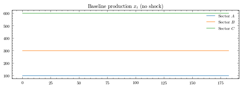
Baseline sectoral output – the system is initialised at a closed input-output equilibrium, so \(x_t = x_0\) for all \(t\).
fig, ax = plt.subplots(figsize=(8, 3))
for name in ["A", "B", "C"]:
    ax.plot(baseline.index, baseline["GrossOutput", name], label=rf"Sector ${name}$")
ax.set_title(r"Baseline production $x_t$ (no shock)")
ax.legend()
plt.tight_layout()
plt.show()
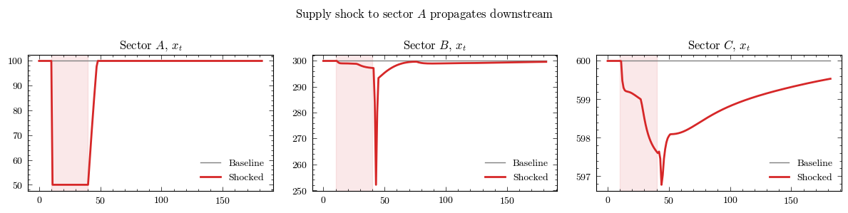
Apply a 50% supply shock to sector A for 30 days starting on day 10 and re-simulate. Sector A’s output drops directly; sectors B and C fall through the essential-input chain \(A \to B \to C\).
shock = {"SupplyShock": torch.zeros(model.parameters.hyper["timesteps"], 3)}
shock["SupplyShock"][10:40, 0] = 0.5
model.scenarios.add_vector_scenario(shock, name="UpstreamShock")
model.simulate(scenario=1)
shocked = model.variables.to_pandas()
Side-by-side comparison: baseline (grey) vs upstream shock (red). Sector \(A\) absorbs the shock immediately; sectors \(B\) and \(C\) drop only modestly during the shock window because their inventories of upstream inputs cushion the supply restriction.
The deeper trough in sector \(B\) around \(t=43\), three days after the shock ends, is the model’s characteristic feature. Three coupled mechanisms drive it.
A’s labour was fired during the shock. When \(A\)’s productive capacity collapsed to 50, the asymmetric labour rule (Eq. 19-20) fired workers down from 60 to 30 to match.
A’s recovery is slow. The default hiring rate is \(\gamma_H = 1/30\) per day. Once the shock ends at \(t=40\), \(A\)’s capacity rebuilds linearly at about seven units per day (50, 57, 64, 71, …) and only returns to 100 around \(t=50\).
B exhausts its \(A\)-input inventory before \(A\) can resupply. During the shock \(B\) kept ordering at near-steady-state level while \(A\) delivered only 50. \(B\)’s on-hand inventory of \(A\)’s output drained to a thin buffer by \(t=40\). In the days after, \(A\) still produces well below \(B\)’s orders, \(B\)’s input capacity falls from \(\approx 460\) to \(\approx 250\), and at \(t=43\) \(B\)’s output is input-bound at 252, a 16% drop below steady state. The input shortage then triggers \(B\)’s own labour adjustment: asymmetric firing (\(\gamma_F = 2/30\)) cuts \(B\)’s capacity, so even after \(A\) recovers around \(t=50\), \(B\)’s production is capped by its reduced workforce until the slower hiring loop rebuilds it.
fig, axs = plt.subplots(ncols=3, figsize=(12, 3))
for ax, name in zip(axs, ["A", "B", "C"]):
    ax.plot(
        baseline.index,
        baseline["GrossOutput", name],
        color="grey",
        linewidth=1,
        label="Baseline",
    )
    ax.plot(
        shocked.index,
        shocked["GrossOutput", name],
        color="tab:red",
        linewidth=2,
        label="Shocked",
    )
    ax.axvspan(10, 40, color="tab:red", alpha=0.1)
    ax.set_title(rf"Sector ${name}$, $x_t$")
    ax.legend()
fig.suptitle(r"Supply shock to sector $A$ propagates downstream")
plt.tight_layout()
plt.show()
Replicating the paper’s results using data#
The Pichler et al. (2022) calibration uses the WIOD UK 2014 55-sector input-output table, the IHS Markit critical-input matrix, and ONS inventory-target ratios. Neither WIOD nor IHS Markit can be redistributed inside this package; users must obtain them under their own licence terms.
The cells below execute only when the PICHLER2022_DATA_DIR
environment variable points to a replication directory; otherwise
they no-op and the rendered public docs show no output for this
section. Set the variable to the parent of data/ and re-run.
Data sources#
Layout expected by from_wiod_uk:
$PICHLER2022_DATA_DIR/
└── data/
    ├── io_data_detail/
    │   ├── GBR_A.csv              # WIOD 55-sector A matrix
    │   ├── GBR_Z.csv              # intermediate consumption Z
    │   ├── GBR_x.csv              # initial gross output
    │   ├── GBR_lab.csv            # labour compensation
    │   ├── GBR_cap.csv            # capital / profits
    │   ├── GBR_f.csv              # final demand
    │   ├── GBR_f_imported.csv     # imported final demand
    │   ├── GBR_consumer_taxes.csv
    │   ├── GBR_firm_taxes.csv
    │   ├── GBR_other_expenses.csv
    │   └── GBR_Z_imports.csv
    ├── IHS_matrices_processed/
    │   └── A.essential2.csv       # IHS Markit critical-input mask
    ├── ons_table_ratio_inv_go.csv # ONS inventory-target days
    └── shocks/
        └── shock_scenarios.csv    # pandemic supply-shock series
WIOD 2016 release (2014 reference year): as of 2026 the canonical project page redirects intermittently; the FIGARO release from Eurostat is a successor product with comparable structure.
IHS Markit critical-input matrix: published as supplementary material with Pichler et al. (2022); check the journal’s replication archive on Zenodo.
ONS inventory ratios: ONS public release.
DATA_ROOT = os.environ.get("PICHLER2022_DATA_DIR")
HAS_DATA = DATA_ROOT is not None and Path(DATA_ROOT).is_dir()
Construct the 55-sector calibration from CSV and attach the paper’s
pandemic shock scenario. Skipped when PICHLER2022_DATA_DIR is
unset.
if HAS_DATA:
    data_dir = Path(DATA_ROOT) / "data" / "io_data_detail"
    ihs_dir = Path(DATA_ROOT) / "data" / "IHS_matrices_processed"
    inv_file = Path(DATA_ROOT) / "data" / "ons_table_ratio_inv_go.csv"
    shock_csv = Path(DATA_ROOT) / "data" / "shocks" / "shock_scenarios.csv"
    fd_csv = data_dir / "GBR_f.csv"

    params = ParametersPichlerEtAl2022DIO.from_wiod_uk(
        data_dir=data_dir, ihs_dir=ihs_dir, inv_file=inv_file
    )
    scenarios = ScenariosPichlerEtAl2022DIO.from_shocks_csv(
        parameters=params, shock_csv=shock_csv, final_demand_csv=fd_csv
    )
    full_model = PichlerEtAl2022DIO(parameters=params, scenarios=scenarios)
    full_model.simulate(scenario=0)
    baseline_full = full_model.variables.to_pandas()
    full_model.simulate(scenario=1)
    shocked_full = full_model.variables.to_pandas()
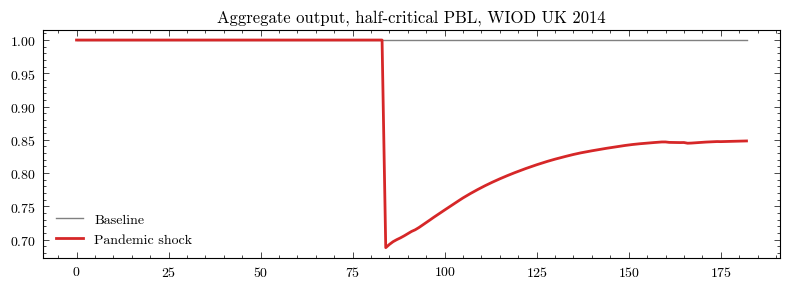
Aggregate gross output, baseline vs pandemic shock, normalised to pre-shock levels. Reproduces the qualitative shape of Pichler et al. (2022) Figure 4.
if HAS_DATA:
    agg_baseline = baseline_full["GrossOutput"].sum(axis=1)
    agg_shocked = shocked_full["GrossOutput"].sum(axis=1)
    norm = agg_baseline.iloc[0]
    fig, ax = plt.subplots(figsize=(8, 3))
    ax.plot(
        agg_baseline.index,
        agg_baseline / norm,
        color="grey",
        linewidth=1,
        label="Baseline",
    )
    ax.plot(
        agg_shocked.index,
        agg_shocked / norm,
        color="tab:red",
        linewidth=2,
        label="Pandemic shock",
    )
    ax.set_title(r"Aggregate output, half-critical PBL, WIOD UK 2014")
    ax.legend()
    plt.tight_layout()
    plt.show()
Source#
Pichler, A., Pangallo, M., del Rio-Chanona, R.M., Lafond, F. & Farmer, J.D. (2022). Forecasting the propagation of pandemic shocks with a dynamic input-output model. Journal of Economic Dynamics and Control, 144, 104527. https://doi.org/10.1016/j.jedc.2022.104527