Model LP3#
Model LP3 extends Model LP2 from Chapter 5 of Godley and Lavoie [2006] by making government expenditures endogenous through a fiscal austerity rule. When the deficit-to-GDP ratio (\(PSBR/Y\)) exceeds a threshold, the government cuts spending. This introduces path-dependence — the long-run steady state depends on the history of shocks, not just the structural parameters.
Module Contents#
As with all MacroStat models, LP3 is divided into Variables, Parameters (fixed constants), Scenarios, and the Behavior (model initialization and steps). The module-level documentation can be seen in:
The remainder of this page gives an introduction to the model, notes on how it is implemented in MacroStat and then shows some of the model dynamics by replicating the relevant graphs of Godley and Lavoie (2006).
Model Overview#
Behavioral Equations#
Model LP3 inherits all 20 equations from Model LP2. The exogenous government spending \(G\) of LP2 is replaced by an endogenous fiscal rule, and a new equation tracks the public sector borrowing requirement.
New equation — Fiscal Austerity Rule (equations 5.28–5.31 of GL06):
New equation — Public Sector Borrowing Requirement:
The fiscal rule is symmetric: the government also loosens when the budget is in surplus beyond the threshold. Government spending adjusts gradually at speed \(\beta_g\), not instantaneously.
Transaction Flow Matrix#
Household |
Production |
Government |
CentralBank |
CentralBank |
Total |
|
|---|---|---|---|---|---|---|
Current |
Current |
Current |
Current |
Capital |
||
Consumption Household |
\(-C(t)\) |
\(+C(t)\) |
\(0\) |
|||
Consumption Government |
\(+G(t)\) |
\(-G(t)\) |
\(0\) |
|||
National Income |
\(+Y(t)\) |
\(-Y(t)\) |
\(0\) |
|||
Taxes |
\(-T(t)\) |
\(+T(t)\) |
\(0\) |
|||
Interest On Bills Household |
\(+r_b(t-1) \cdot B_h(t-1)\) |
\(-r_b(t-1) \cdot B_h(t-1)\) |
\(0\) |
|||
Bond Coupon Income Household |
\(+BL_h(t-1)\) |
\(-BL_h(t-1)\) |
\(0\) |
|||
Central Bank Profits |
\(+r_b(t-1) \cdot B_{CB}(t-1)\) |
\(-r_b(t-1) \cdot B_{CB}(t-1)\) |
\(0\) |
|||
Change in Bill Stock |
\(+\Delta B_h(t)\) |
\(-\Delta B_s(t)\) |
\(+\Delta B_{CB}(t)\) |
\(0\) |
||
Change in Bond Stock |
\(+\Delta BL_h(t)\) |
\(0\) |
||||
Change in Bond Supply |
\(-\Delta BL_s(t)\) |
\(0\) |
||||
Change in Cash Stock |
\(+\Delta H_h(t)\) |
\(0\) |
||||
Change in Money Stock |
\(-\Delta H_s(t)\) |
\(0\) |
||||
Total |
\(0\) |
\(0\) |
\(0\) |
\(0\) |
\(0\) |
\(0\) |
Balance Sheet Matrix#
Household |
Production |
Government |
CentralBank |
Total |
|
|---|---|---|---|---|---|
Current |
Current |
Current |
Capital |
||
Wealth |
\(-V(t)\) |
\(+V(t)\) |
0 |
||
Bill Stock |
\(+B_h(t)\) |
\(-B_s(t)\) |
\(+B_{CB}(t)\) |
0 |
|
Bond Stock |
\(+BL_h(t)\) |
0 |
|||
Bond Supply |
\(-BL_s(t)\) |
0 |
|||
Cash Stock |
\(+H_h(t)\) |
0 |
|||
Money Stock |
\(-H_s(t)\) |
0 |
Implementation in MacroStat#
Transposing these equations to the MacroStat framework, we consider that there are:
Eighteen parameters (fixed constants): all sixteen from LP2, plus \(\beta_g\) (fiscal adjustment speed) and \(\phi\) (PSBR threshold) (see Parameters)
One scenario variable: \(r_b(t)\) — both bond prices and government spending are now endogenous (see Scenarios)
The remaining tracked series are variables — including the new
PublicSectorBorrowingRequirement(see Variables)
Model Dynamics#
Preparatory Steps#
%load_ext autoreload
%autoreload 2

import importlib
import logging
import sys

# Import the necessary libraries for plotting
from matplotlib import pyplot as plt
from matplotlib.ticker import PercentFormatter

# Import the MacroStat model components
from macrostat.models.GL06LP import GL06LP, ParametersGL06LP, ScenariosGL06LP
from macrostat.models.GL06LP3 import GL06LP3, ParametersGL06LP3, ScenariosGL06LP3

# Custom matplotlib style for the documentation
plt.style.use("../../macrostat.mplstyle")
# We show the logging output in the notebook
importlib.reload(logging)
logging.basicConfig(stream=sys.stdout, level=logging.INFO)
Running the Simulation#
In LP3, government spending adjusts endogenously after the first period. The initial value \(G_0 = 20\) is used in period 1, then the fiscal rule takes over. The PSBR-to-GDP ratio converges toward zero as the government adjusts spending to balance the budget.
params = ParametersGL06LP3()
model = GL06LP3(parameters=params)
model.simulate()
output = model.variables.to_pandas()
We can check that the variables are healthy, meaning the redundant equation \(H_h = H_s\) holds and all stocks are positive.
Note
Due to floating point precision, the redundant equation will not hold exactly. We check that the absolute percentage error is below a tolerance.
model.variables.check_health(tolerance=1e-3)
True
An overview of the first 10 steps of the model:
df = model.variables.to_pandas()
df.head(10).T
| time | 0 | 1 | 2 | 3 | 4 | 5 | 6 | 7 | 8 | 9 | |
|---|---|---|---|---|---|---|---|---|---|---|---|
| ConsumptionHousehold | Household | 0.0 | 0.0 | 0.000000 | 16.124001 | 28.993177 | 39.686977 | 48.558765 | 55.919319 | 62.026039 | 67.092545 |
| ConsumptionGovernment | Government | 0.0 | 0.0 | 20.000000 | 19.838760 | 19.710068 | 19.603130 | 19.514412 | 19.440807 | 19.379740 | 19.329075 |
| NationalIncome | Macroeconomy | 0.0 | 0.0 | 20.000000 | 35.962761 | 48.703247 | 59.290108 | 68.073181 | 75.360123 | 81.405777 | 86.421616 |
| Taxes | Household | 0.0 | 0.0 | 3.876000 | 6.969583 | 9.540234 | 11.672894 | 13.442276 | 14.910254 | 16.128176 | 17.138641 |
| InterestOnBillsHousehold | Household | 0.0 | 0.0 | 0.000000 | 0.000000 | 0.189307 | 0.341071 | 0.467330 | 0.572079 | 0.658957 | 0.731008 |
| BondCouponIncomeHousehold | Household | 0.0 | 0.0 | 0.000000 | 0.000000 | 0.334654 | 0.600475 | 0.821078 | 1.004089 | 1.155981 | 1.282050 |
| CentralBankProfits | CentralBank | 0.0 | 0.0 | 0.000000 | 0.483720 | 0.487647 | 0.503520 | 0.516294 | 0.526903 | 0.535701 | 0.542999 |
| CapitalGains | Household | 0.0 | 0.0 | -0.000000 | -0.000000 | 0.000000 | 0.000000 | 0.000000 | 0.000000 | 0.000000 | 0.000000 |
| ExpectedCapitalGains | Household | 0.0 | 0.0 | 0.000000 | 0.009906 | 0.008887 | 0.006076 | 0.003715 | 0.002138 | 0.001186 | 0.000641 |
| Wealth | Household | 0.0 | 0.0 | 16.124001 | 28.993179 | 39.686981 | 48.558765 | 55.919315 | 62.026031 | 67.092537 | 71.296036 |
| HouseholdBillStock | Household | 0.0 | 0.0 | 0.000000 | 6.310246 | 11.369034 | 15.577663 | 19.069304 | 21.965221 | 24.366936 | 26.358936 |
| GovernmentBillStock | Government | 0.0 | 0.0 | 16.124001 | 22.565136 | 28.153038 | 32.787479 | 36.632748 | 39.821934 | 42.466904 | 44.660660 |
| CentralBankBillStock | CentralBank | 0.0 | 0.0 | 16.124001 | 16.254890 | 16.784004 | 17.209816 | 17.563444 | 17.856712 | 18.099968 | 18.301723 |
| HouseholdBondStock | Household | 0.0 | 0.0 | 0.000000 | 0.334654 | 0.600475 | 0.821078 | 1.004089 | 1.155981 | 1.282050 | 1.386680 |
| GovernmentBondSupply | Government | 0.0 | 0.0 | 0.000000 | 0.334654 | 0.600475 | 0.821078 | 1.004089 | 1.155981 | 1.282050 | 1.386680 |
| HouseholdCashStock | Household | 0.0 | 0.0 | 16.124001 | 16.254892 | 16.784016 | 17.209831 | 17.563463 | 17.856722 | 18.099981 | 18.301744 |
| CentralBankMoneyStock | CentralBank | 0.0 | 0.0 | 16.124001 | 16.254890 | 16.784004 | 17.209816 | 17.563446 | 17.856714 | 18.099968 | 18.301723 |
| DisposableIncome | Household | 0.0 | 0.0 | 16.124001 | 28.993177 | 39.686977 | 48.558762 | 55.919315 | 62.026035 | 67.092545 | 71.296036 |
| ExpectedDisposableIncome | Household | 0.0 | 0.0 | 0.000000 | 16.124001 | 28.993177 | 39.686977 | 48.558762 | 55.919315 | 62.026035 | 67.092545 |
| ExpectedWealth | Household | 0.0 | 0.0 | 0.000000 | 16.124001 | 28.993181 | 39.686985 | 48.558758 | 55.919312 | 62.026024 | 67.092545 |
| HouseholdBillDemand | Household | 0.0 | 0.0 | 0.000000 | 6.310246 | 11.369034 | 15.577663 | 19.069304 | 21.965221 | 24.366936 | 26.358936 |
| HouseholdBondDemand | Household | 0.0 | 0.0 | 0.000000 | 0.334654 | 0.600475 | 0.821078 | 1.004089 | 1.155981 | 1.282050 | 1.386680 |
| HouseholdCashDemand | Household | 0.0 | 0.0 | 0.000000 | 3.385713 | 6.090216 | 8.338050 | 10.202904 | 11.750002 | 13.033468 | 14.098253 |
| InterestRateBills | Macroeconomy | 0.0 | 0.0 | 0.030000 | 0.030000 | 0.030000 | 0.030000 | 0.030000 | 0.030000 | 0.030000 | 0.030000 |
| BondPrice | Macroeconomy | 20.0 | 20.0 | 19.600000 | 19.208000 | 19.208000 | 19.208000 | 19.208000 | 19.208000 | 19.208000 | 19.208000 |
| BondYield | Macroeconomy | 0.0 | 0.0 | 0.051020 | 0.052062 | 0.052062 | 0.052062 | 0.052062 | 0.052062 | 0.052062 | 0.052062 |
| ExpectedBondPrice | Household | 20.0 | 20.0 | 19.799999 | 19.504000 | 19.355999 | 19.282000 | 19.244999 | 19.226500 | 19.217251 | 19.212626 |
| ExpectedReturnOnBonds | Household | 0.0 | 0.0 | 0.052041 | 0.053603 | 0.052832 | 0.052447 | 0.052254 | 0.052158 | 0.052110 | 0.052086 |
| TargetProportion | Government | 0.0 | 0.0 | 0.000000 | 0.000000 | 0.504624 | 0.503600 | 0.503088 | 0.502832 | 0.502704 | 0.502640 |
| PublicSectorBorrowingRequirement | Government | 0.0 | 0.0 | 16.124001 | 12.869179 | 10.693795 | 8.871782 | 7.360544 | 6.106721 | 5.066502 | 4.203491 |
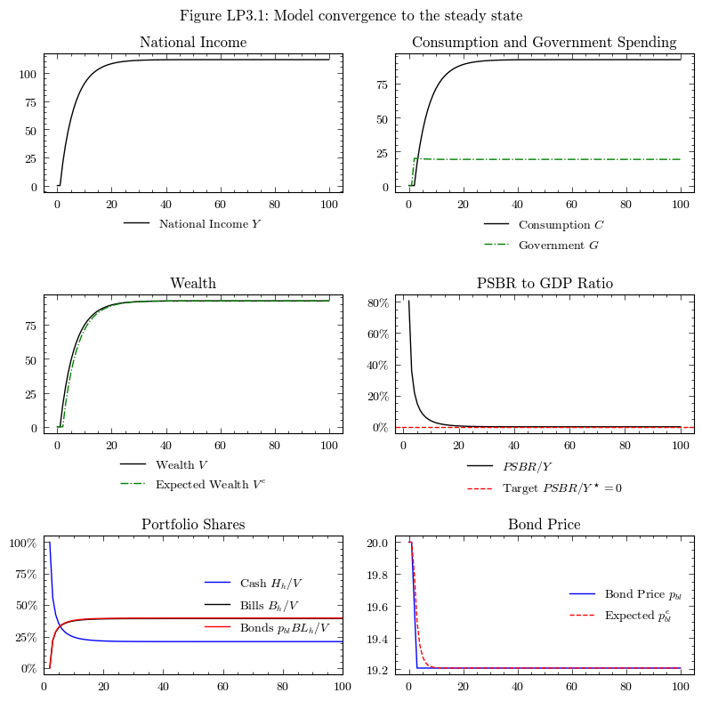
Convergence to the Steady State#
In the steady state of Model LP3, the fiscal rule drives \(PSBR/Y \to 0\). Government spending adjusts slowly (governed by \(\beta_g\)) until the budget is balanced. The long-run outcome is similar to LP2 in terms of portfolio composition, but the level of government spending (and hence income) is path-dependent.
dfo = output.loc[:100]

fig, axs = plt.subplots(ncols=2, nrows=3, figsize=(8, 8))

# National Income
axs[0, 0].plot(dfo.index, dfo['NationalIncome'], color='k', label=r'National Income $Y$')
axs[0, 0].legend(loc='upper center', bbox_to_anchor=(0.5, -0.1), frameon=False)
axs[0, 0].set_title('National Income')

# Consumption and Government Spending
axs[0, 1].plot(dfo.index, dfo['ConsumptionHousehold'], color='k', label=r'Consumption $C$')
axs[0, 1].plot(dfo.index, dfo['ConsumptionGovernment'], color='g', linestyle='-.', label=r'Government $G$')
axs[0, 1].legend(loc='upper center', bbox_to_anchor=(0.5, -0.1), frameon=False)
axs[0, 1].set_title('Consumption and Government Spending')

# Wealth
axs[1, 0].plot(dfo.index, dfo['Wealth'], color='k', label=r'Wealth $V$')
axs[1, 0].plot(dfo.index, dfo['ExpectedWealth'], color='g', linestyle='-.', label=r'Expected Wealth $V^e$')
axs[1, 0].legend(loc='upper center', bbox_to_anchor=(0.5, -0.1), frameon=False)
axs[1, 0].set_title('Wealth')

# PSBR / Y ratio
psbr_ratio = output['PublicSectorBorrowingRequirement'].div(output['NationalIncome']['Macroeconomy'], axis=0)
axs[1, 1].plot(dfo.index, psbr_ratio.loc[:100], color='k', label=r'$PSBR/Y$')
axs[1, 1].axhline(y=0, color='r', linestyle='--', label=r'Target $PSBR/Y^\star=0$')
axs[1, 1].legend(loc='upper center', bbox_to_anchor=(0.5, -0.1), frameon=False)
axs[1, 1].set_title('PSBR to GDP Ratio')
axs[1, 1].yaxis.set_major_formatter(PercentFormatter(1))

# Portfolio Shares
cash_share = output['HouseholdCashStock'] / output['Wealth']
bill_share = output['HouseholdBillStock'] / output['Wealth']
bond_share = (output['HouseholdBondStock'].mul(output[('BondPrice','Macroeconomy')], axis=0)) / output['Wealth']

axs[2, 0].plot(output.index, cash_share, color='b', label='Cash $H_h/V$')
axs[2, 0].plot(output.index, bill_share, color='k', label='Bills $B_h/V$')
axs[2, 0].plot(output.index, bond_share, color='r', label='Bonds $p_{bl} BL_h/V$')
axs[2, 0].legend(loc='center right', frameon=False)
axs[2, 0].set_xlim(0, 100)
axs[2, 0].set_title('Portfolio Shares')
axs[2, 0].yaxis.set_major_formatter(PercentFormatter(1))

# Bond Price
axs[2, 1].plot(dfo.index, dfo[('BondPrice', 'Macroeconomy')], color='b', label=r'Bond Price $p_{bl}$')
axs[2, 1].plot(dfo.index, dfo['ExpectedBondPrice'], color='r', linestyle='--', label=r'Expected $p_{bl}^e$')
axs[2, 1].legend(loc='center right', frameon=False)
axs[2, 1].set_title('Bond Price')

fig.suptitle('Figure LP3.1: Model convergence to the steady state')
plt.tight_layout()
plt.show()
Perturbation 1: Drop in Propensity to Consume (Section 5.9, Figure 5.10 vs 5.11)#
Following Section 5.9 of Godley and Lavoie [2006], we reduce the propensity to consume out of current income (\(\alpha_1\)) by 0.1. This induces a recession that raises the government deficit (lower taxes, same spending). In LP (with exogenous G), the economy recovers above its initial level. In LP3, the fiscal austerity rule kicks in: once \(PSBR/Y\) exceeds the threshold, government spending is cut, deepening and prolonging the recession.
We run both LP3 and LP (for comparison) with the same \(\alpha_1\) shock:
# Run LP3 with the drop in alpha1
scenarios_lp3 = ScenariosGL06LP3(parameters=params)
sc1 = scenarios_lp3.get_scenario_index("Scenario.1: Drop in alpha1")
model1 = GL06LP3(parameters=params, scenarios=scenarios_lp3)
model1.simulate(scenario=sc1)
output_sc1 = model1.variables.to_pandas()

# Run LP (exogenous G) for comparison — same alpha1 shock
params_lp = ParametersGL06LP()
scenarios_lp = ScenariosGL06LP(parameters=params_lp)
sc_lp = scenarios_lp.get_scenario_index("Scenario.2: Drop in alpha1")
model_lp_base = GL06LP(parameters=params_lp)
model_lp_base.simulate()
output_lp1_base = model_lp_base.variables.to_pandas()
model_lp1 = GL06LP(parameters=params_lp, scenarios=scenarios_lp)
model_lp1.simulate(scenario=sc_lp)
output_lp1_shock = model_lp1.variables.to_pandas()
trigger = params["scenario_trigger"]

fig, axes = plt.subplots(1, 2, figsize=(12, 4), sharey=True)

# Figure 5.10 (LP — exogenous G)
ax = axes[0]
ax.plot(output_lp1_base.loc[trigger - 2:].index,
        output_lp1_base.loc[trigger - 2:, 'NationalIncome'], 'k--', label='Baseline')
ax.plot(output_lp1_shock.loc[trigger - 2:].index,
        output_lp1_shock.loc[trigger - 2:, 'NationalIncome'], 'k-', label='Shock')
ax.axvline(x=trigger, color='grey', linestyle=':', alpha=0.5)
ax.set_title('Figure 5.10: $Y$ in Model LP (exogenous $G$)')
ax.set_xlabel('Period')
ax.legend(frameon=False)

# Figure 5.11 (LP3 — fiscal rule)
ax = axes[1]
ax.plot(output.loc[trigger - 2:].index,
        output.loc[trigger - 2:, 'NationalIncome'], 'k--', label='Baseline (LP3)')
ax.plot(output_sc1.loc[trigger - 2:].index,
        output_sc1.loc[trigger - 2:, 'NationalIncome'], 'k-', label='Shock (LP3)')
ax.axvline(x=trigger, color='grey', linestyle=':', alpha=0.5)
ax.set_title('Figure 5.11: $Y$ in Model LP3 (fiscal rule)')
ax.set_xlabel('Period')
ax.legend(frameon=False)

fig.suptitle('Figures 5.10 & 5.11: Drop in $\\alpha_1$ - LP vs LP3 (fiscal rule)')
plt.tight_layout()
plt.show()
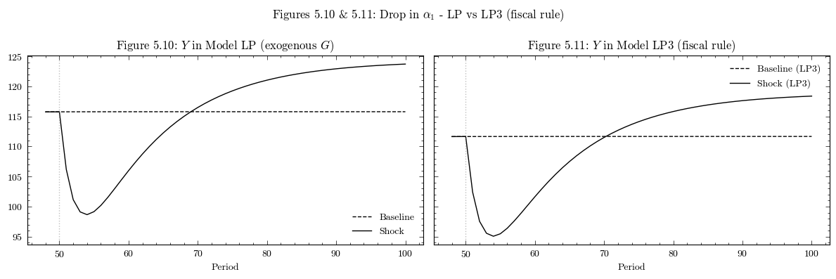
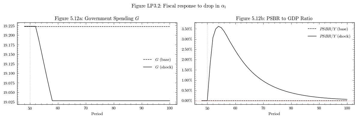
Figure 5.12: Government expenditures and the PSBR-to-GDP ratio. Once the threshold is breached, government spending is cut each period until the ratio returns within bounds.
dfo = output_sc1.loc[trigger - 2:]
dfo_base = output.loc[trigger - 2:]

fig, axes = plt.subplots(1, 2, figsize=(12, 4))

# Government spending
ax = axes[0]
ax.plot(dfo_base.index, dfo_base['ConsumptionGovernment'], 'k--', label='$G$ (base)')
ax.plot(dfo.index, dfo['ConsumptionGovernment'], 'k-', label='$G$ (shock)')
ax.axvline(x=trigger, color='grey', linestyle=':', alpha=0.5)
ax.set_title('Figure 5.12a: Government Spending $G$')
ax.set_xlabel('Period')
ax.legend(frameon=False)

# PSBR / Y
psbr_base = dfo_base['PublicSectorBorrowingRequirement'].div(dfo_base['NationalIncome']['Macroeconomy'], axis=0)
psbr_shock = dfo['PublicSectorBorrowingRequirement'].div(dfo['NationalIncome']['Macroeconomy'],axis=0)
ax = axes[1]
ax.plot(dfo_base.index, psbr_base, 'k--', label='$PSBR/Y$ (base)')
ax.plot(dfo.index, psbr_shock, 'k-', label='$PSBR/Y$ (shock)')
ax.axhline(y=0, color='r', linestyle=':', alpha=0.5)
ax.axvline(x=trigger, color='grey', linestyle=':', alpha=0.5)
ax.set_title('Figure 5.12b: PSBR to GDP Ratio')
ax.set_xlabel('Period')
ax.yaxis.set_major_formatter(PercentFormatter(1))
ax.legend(frameon=False)

fig.suptitle('Figure LP3.2: Fiscal response to drop in $\\alpha_1$')
plt.tight_layout()
plt.show()
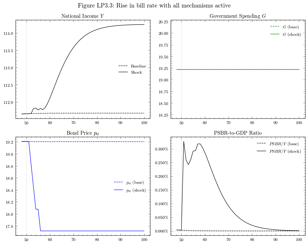
Perturbation 2: Rise in Bill Rate (all mechanisms active)#
In this experiment, we raise the Treasury bill rate from 3% to 4% in a model where all three LP3 mechanisms are active: Tobin portfolio choice, endogenous bond prices, and the fiscal rule. The bill rate rise makes bills more attractive, reallocates the portfolio, pushes up the bond price endogenously, and increases government debt service costs, potentially triggering the fiscal rule.
scenarios_lp3_2 = ScenariosGL06LP3(parameters=params)
sc2 = scenarios_lp3_2.get_scenario_index("Scenario.2: Rise in bill rate")
model2 = GL06LP3(parameters=params, scenarios=scenarios_lp3_2)
model2.simulate(scenario=sc2)
output_sc2 = model2.variables.to_pandas()
dfo2 = output_sc2.loc[trigger - 2:]

fig, axes = plt.subplots(2, 2, figsize=(10, 8))
fig.suptitle('Figure LP3.3: Rise in bill rate with all mechanisms active', fontsize=14)

# National Income
axes[0, 0].plot(dfo_base.index, dfo_base['NationalIncome'], 'k--', label='Baseline')
axes[0, 0].plot(dfo2.index, dfo2['NationalIncome'], 'k-', label='Shock')
axes[0, 0].axvline(x=trigger, color='grey', linestyle=':', alpha=0.5)
axes[0, 0].set_title('National Income $Y$')
axes[0, 0].legend(frameon=False)

# Government Spending
axes[0, 1].plot(dfo_base.index, dfo_base['ConsumptionGovernment'], 'g--', label='$G$ (base)')
axes[0, 1].plot(dfo2.index, dfo2['ConsumptionGovernment'], 'g-', label='$G$ (shock)')
axes[0, 1].axvline(x=trigger, color='grey', linestyle=':', alpha=0.5)
axes[0, 1].set_title('Government Spending $G$')
axes[0, 1].legend(frameon=False)

# Bond Price
axes[1, 0].plot(dfo_base.index, dfo_base[('BondPrice','Macroeconomy')], 'b--', label='$p_{bl}$ (base)')
axes[1, 0].plot(dfo2.index, dfo2[('BondPrice','Macroeconomy')], 'b-', label='$p_{bl}$ (shock)')
axes[1, 0].axvline(x=trigger, color='grey', linestyle=':', alpha=0.5)
axes[1, 0].set_title('Bond Price $p_{bl}$')
axes[1, 0].legend(frameon=False)

# PSBR / Y
psbr_base2 = dfo_base['PublicSectorBorrowingRequirement'].div(dfo_base['NationalIncome']['Macroeconomy'], axis=0)
psbr_sc2 = dfo2['PublicSectorBorrowingRequirement'].div(dfo2['NationalIncome']['Macroeconomy'], axis=0)
axes[1, 1].plot(dfo_base.index, psbr_base2, 'k--', label='$PSBR/Y$ (base)')
axes[1, 1].plot(dfo2.index, psbr_sc2, 'k-', label='$PSBR/Y$ (shock)')
axes[1, 1].axhline(y=0, color='r', linestyle=':', alpha=0.5)
axes[1, 1].axvline(x=trigger, color='grey', linestyle=':', alpha=0.5)
axes[1, 1].set_title('PSBR-to-GDP Ratio')
axes[1, 1].yaxis.set_major_formatter(PercentFormatter(1))
axes[1, 1].legend(frameon=False)

plt.tight_layout()
plt.show()