Model PC#
Model PC is introduced in chapter 4 of Godley and Lavoie [2006] “Monetary Economics: An Integrated Approach to Credit, Money, Income, Production and Wealth”.
Module Contents#
As with all MacroStat models, PC is divided into Variables, Parameters (fixed constants), Scenarios, and the Behavior (model initialization and steps). The module-level documentation, such as all variables/parameters/scenarios and their notation or the behavioral equations associated with each function of BehaviorPC.py can be seen in:
The remainder of this page gives an introduction to the model, notes on how it is implemented in MacroStat and then shows some of the model dynamics by replicating the relevant graphs of Godley and Lavoie (2006).
Model Overview#
Transaction Flow Matrix#
Household |
Production |
Government |
CentralBank |
CentralBank |
Total |
|
|---|---|---|---|---|---|---|
Current |
Current |
Current |
Current |
Capital |
||
Consumption Household |
\(-C(t)\) |
\(+C(t)\) |
\(0\) |
|||
Consumption Government |
\(+G(t)\) |
\(-G(t)\) |
\(0\) |
|||
National Income |
\(+Y(t)\) |
\(-Y(t)\) |
\(0\) |
|||
Interest Earned On Bills Household |
\(+r(t-1)\cdot B_h(t-1)\) |
\(-r(t-1)\cdot B_h(t-1)\) |
\(0\) |
|||
Central Bank Profits |
\(+r(t-1)\cdot B_{CB}(t-1)\) |
\(-r(t-1)\cdot B_{CB}(t-1)\) |
\(0\) |
|||
Taxes |
\(-T(t)\) |
\(+T(t)\) |
\(0\) |
|||
Change in Money Stock |
\(+\Delta H_h(t)\) |
\(-\Delta H_{s}(t)\) |
\(0\) |
|||
Change in Bill Stock |
\(+\Delta B_h(t)\) |
\(-\Delta B_s(t)\) |
\(+\Delta B_{CB}(t)\) |
\(0\) |
||
Total |
\(0\) |
\(0\) |
\(0\) |
\(0\) |
\(0\) |
\(0\) |
Balance Sheet Matrix#
Household |
Production |
Government |
CentralBank |
Total |
|
|---|---|---|---|---|---|
Current |
Current |
Current |
Capital |
||
Money Stock |
\(+H_h(t)\) |
\(-H_{s}(t)\) |
0 |
||
Bill Stock |
\(+B_h(t)\) |
\(-B_s(t)\) |
\(+B_{CB}(t)\) |
0 |
|
Wealth |
\(-V(t)\) |
\(+V(t)\) |
0 |
Implementation in MacroStat#
Transposing these eleven equations to the MacroStat framework, we consider that there are:
Three parameters (fixed constants): \(\alpha_1\), \(\alpha_2\), and \(\theta\) (see Parameters)
Two scenario variables : \(G_d(t)\) and \(W(t)\) (see Scenarios)
The remaining 14 tracked series are variables (see Variables)
Behavioral Modeling#
The model PC imposes that the assumptions of the household on income are correct and firms supply all goods. For the implementation of the behavioral equations (see Behavior), most prior implementations have made use of some form of linear solver or iteration until the system is solved. To simplify the implementation in Macrostat, we can note that the system can be solved analytically for a given timestep as follows:
Substitute the consumption equation into the national income equation to obtain
where \(G(t)\) is exogenous and \(V(t-1)\) is determined. Substituting further the disposable income equation and tax equation we can obtain
which can be rearranged to yield a solution for \(Y(t)\)
Therefore, for a given period \(t\) we can solve the system by solving, in order:
Eq. (1) for national income \(Y(t)\)
Eq.
gl06_pc_eq403_taxesfor taxes \(T(t)\)Eq.
gl06_pc_eq402_disposableIncomefor disposable income \(YD(t)\)Eq.
gl06_pc_eq405_consumptionfor consumption \(C(t)\)Eq.
gl06_pc_eq404_wealthfor wealth \(V(t)\)Eq.
gl06_pc_eq407_householdBondHoldingsfor household bill holdings \(B_h(t)\)Eq.
gl06_pc_eq406_householdDepositsfor household depositis (residual) \(H_h(t)\)Eq.
gl06_pc_eq408_governmentBillIssuancefor the government budget resulting in bill issuance \(B_s(t)\)Eq.
gl06_pc_eq410_centralBankBillsfor the Central Bank holding of bills \(B_{CB}(t)\)Eq.
gl06_pc_eq409_moneyIssuancefor the level of cash money \(H_s(t)\)
This is implemented as such in the Behavior class.
Model Dynamics#
Preparatory Steps#
%load_ext autoreload
%autoreload 2

import importlib
import logging
import sys

# Import the necessary libraries for plotting
from matplotlib import pyplot as plt
from matplotlib.ticker import PercentFormatter

# Import the MacroStat get_model function
from macrostat.models import get_model

# Custom matplotlib style for the documentation
plt.style.use("../../macrostat.mplstyle")
# We show the logging output in the notebook
importlib.reload(logging)
logging.basicConfig(stream=sys.stdout, level=logging.INFO)
Running the Simulation#
First, we can run the model without any shocks to see the convergence to the steady state.
GL06PCClass = get_model("GL06PC")
model = GL06PCClass()
model.simulate()
output = model.variables.to_pandas()
INFO:root:Starting simulation. Scenario: 0
Here we can also check that the variables are healthy, which means that the redundant equations hold and that all the assets and liabilities are positive. For model PC, the redundant equation is that the household money stock equals the central bank money stock.
Note
In numerical implementations, due to floating point precision it is unlikely that the redundant equation will hold exactly. Therefore, we check that the absolute percentage error is less than a given tolerance, in this case 1e-5. We use the absolute percentage error to appropriately scale the error for different magnitudes of the variables.
model.variables.check_health(tolerance=1e-5)
True
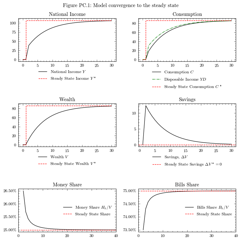
Convergence to the Steady State#
Following the derivations of section 4.5 in Godley and Lavoie [2006], we compute the steady state as
model.compute_theoretical_steady_state(scenario=0)
steadystate = model.variables.to_pandas()
INFO:root:Computing theoretical steady state. Scenario: 0