Model LP2#
Model LP2 extends Model LP from Chapter 5 of Godley and Lavoie [2006] by making bond prices endogenous through a target-proportion mechanism and replacing static bond-price expectations with adaptive expectations. In all other respects, LP2 inherits the equations of LP unchanged.
Module Contents#
As with all MacroStat models, LP2 is divided into Variables, Parameters (fixed constants), Scenarios, and the Behavior (model initialization and steps). The module-level documentation can be seen in:
The remainder of this page gives an introduction to the model, notes on how it is implemented in MacroStat and then shows some of the model dynamics by replicating the relevant graphs of Godley and Lavoie (2006).
Model Overview#
Behavioral Equations#
Model LP2 inherits equations 1–9 and 13–20 unchanged from Model LP. The static-expectations equation (\(p_{bl}^e = p_{bl}\), equation 10 in LP) is replaced by two new equations that make bond prices endogenous and expectations adaptive.
New equation 10a — Target Proportion:
New equation 10b — Endogenous Bond Price:
New equation 10d — Adaptive Expectations:
With adaptive expectations, the expected capital gain \(\chi \cdot (p_{bl}^e - p_{bl})/p_{bl}\) in the expected return on bonds \(ERr_{bl}\) is no longer zero at each period, generating richer portfolio dynamics than in LP.
Transaction Flow Matrix#
Household |
Production |
Government |
CentralBank |
CentralBank |
Total |
|
|---|---|---|---|---|---|---|
Current |
Current |
Current |
Current |
Capital |
||
Consumption Household |
\(-C(t)\) |
\(+C(t)\) |
\(0\) |
|||
Consumption Government |
\(+G(t)\) |
\(-G(t)\) |
\(0\) |
|||
National Income |
\(+Y(t)\) |
\(-Y(t)\) |
\(0\) |
|||
Taxes |
\(-T(t)\) |
\(+T(t)\) |
\(0\) |
|||
Interest On Bills Household |
\(+r_b(t-1) \cdot B_h(t-1)\) |
\(-r_b(t-1) \cdot B_h(t-1)\) |
\(0\) |
|||
Bond Coupon Income Household |
\(+BL_h(t-1)\) |
\(-BL_h(t-1)\) |
\(0\) |
|||
Central Bank Profits |
\(+r_b(t-1) \cdot B_{CB}(t-1)\) |
\(-r_b(t-1) \cdot B_{CB}(t-1)\) |
\(0\) |
|||
Change in Bill Stock |
\(+\Delta B_h(t)\) |
\(-\Delta B_s(t)\) |
\(+\Delta B_{CB}(t)\) |
\(0\) |
||
Change in Bond Stock |
\(+\Delta BL_h(t)\) |
\(0\) |
||||
Change in Bond Supply |
\(-\Delta BL_s(t)\) |
\(0\) |
||||
Change in Cash Stock |
\(+\Delta H_h(t)\) |
\(0\) |
||||
Change in Money Stock |
\(-\Delta H_s(t)\) |
\(0\) |
||||
Total |
\(0\) |
\(0\) |
\(0\) |
\(0\) |
\(0\) |
\(0\) |
Balance Sheet Matrix#
Household |
Production |
Government |
CentralBank |
Total |
|
|---|---|---|---|---|---|
Current |
Current |
Current |
Capital |
||
Wealth |
\(-V(t)\) |
\(+V(t)\) |
0 |
||
Bill Stock |
\(+B_h(t)\) |
\(-B_s(t)\) |
\(+B_{CB}(t)\) |
0 |
|
Bond Stock |
\(+BL_h(t)\) |
0 |
|||
Bond Supply |
\(-BL_s(t)\) |
0 |
|||
Cash Stock |
\(+H_h(t)\) |
0 |
|||
Money Stock |
\(-H_s(t)\) |
0 |
Implementation in MacroStat#
Transposing these equations to the MacroStat framework, we consider that there are:
Sixteen parameters (fixed constants): \(\alpha_1\), \(\alpha_2\), \(\theta\), \(\chi\), the eight \(\lambda\) portfolio coefficients, \(\beta\) (bond price adjustment step), \(\beta_e\) (expectation adjustment speed), \(\text{top}\) (upper target proportion bound), and \(\text{bot}\) (lower target proportion bound) (see Parameters)
Two scenario variables: \(G(t)\) and \(r_b(t)\) — bond prices are now endogenous (see Scenarios)
The remaining tracked series are variables — including the new
TargetProportionandExpectedBondPrice(see Variables)
Model Dynamics#
Preparatory Steps#
%load_ext autoreload
%autoreload 2

import importlib
import logging
import sys

# Import the necessary libraries for plotting
from matplotlib import pyplot as plt
from matplotlib.ticker import PercentFormatter

# Import the MacroStat model components
from macrostat.models.GL06LP2 import GL06LP2, ParametersGL06LP2, ScenariosGL06LP2

# Custom matplotlib style for the documentation
plt.style.use("../../macrostat.mplstyle")
# We show the logging output in the notebook
importlib.reload(logging)
logging.basicConfig(stream=sys.stdout, level=logging.INFO)
Running the Simulation#
First, we run the model without any shocks to see the convergence to the steady state.
params = ParametersGL06LP2()
model = GL06LP2(parameters=params)
model.simulate()
output = model.variables.to_pandas()
We can check that the variables are healthy, meaning the redundant equation \(H_h = H_s\) holds and all stocks are positive.
Note
Due to floating point precision, the redundant equation will not hold exactly. We check that the absolute percentage error is below a tolerance.
model.variables.check_health(tolerance=1e-3)
True
An overview of the first 10 steps of the model:
df = model.variables.to_pandas()
df.head(10).T
| time | 0 | 1 | 2 | 3 | 4 | 5 | 6 | 7 | 8 | 9 | |
|---|---|---|---|---|---|---|---|---|---|---|---|
| ConsumptionHousehold | Household | 0.0 | 0.0 | 0.000000 | 16.124001 | 29.123171 | 40.025520 | 49.155052 | 56.800381 | 63.202782 | 68.564339 |
| ConsumptionGovernment | Government | 0.0 | 0.0 | 20.000000 | 20.000000 | 20.000000 | 20.000000 | 20.000000 | 20.000000 | 20.000000 | 20.000000 |
| NationalIncome | Macroeconomy | 0.0 | 0.0 | 20.000000 | 36.124001 | 49.123169 | 60.025520 | 69.155052 | 76.800385 | 83.202782 | 88.564339 |
| Taxes | Household | 0.0 | 0.0 | 3.876000 | 7.000832 | 9.621614 | 11.816236 | 13.654072 | 15.193127 | 16.481977 | 17.561300 |
| InterestOnBillsHousehold | Household | 0.0 | 0.0 | 0.000000 | 0.000000 | 0.189307 | 0.342600 | 0.471316 | 0.579104 | 0.669339 | 0.744877 |
| BondCouponIncomeHousehold | Household | 0.0 | 0.0 | 0.000000 | 0.000000 | 0.334654 | 0.603168 | 0.828082 | 1.016420 | 1.174195 | 1.306373 |
| CentralBankProfits | CentralBank | 0.0 | 0.0 | 0.000000 | 0.483720 | 0.491546 | 0.510596 | 0.526161 | 0.539205 | 0.550126 | 0.559269 |
| CapitalGains | Household | 0.0 | 0.0 | -0.000000 | -0.000000 | 0.000000 | 0.000000 | 0.000000 | 0.000000 | 0.000000 | 0.000000 |
| ExpectedCapitalGains | Household | 0.0 | 0.0 | 0.000000 | 0.009906 | 0.008927 | 0.006128 | 0.003761 | 0.002172 | 0.001208 | 0.000655 |
| Wealth | Household | 0.0 | 0.0 | 16.124001 | 29.123169 | 40.025520 | 49.155052 | 56.800377 | 63.202778 | 68.564339 | 73.054283 |
| HouseholdBillStock | Household | 0.0 | 0.0 | 0.000000 | 6.310246 | 11.420005 | 15.710543 | 19.303473 | 22.311302 | 24.829226 | 26.937166 |
| GovernmentBillStock | Government | 0.0 | 0.0 | 16.124001 | 22.695127 | 28.439871 | 33.249241 | 37.276981 | 40.648834 | 43.471512 | 45.834629 |
| CentralBankBillStock | CentralBank | 0.0 | 0.0 | 16.124001 | 16.384880 | 17.019867 | 17.538698 | 17.973509 | 18.337532 | 18.642286 | 18.897463 |
| HouseholdBondStock | Household | 0.0 | 0.0 | 0.000000 | 0.334654 | 0.603168 | 0.828082 | 1.016420 | 1.174195 | 1.306373 | 1.417100 |
| GovernmentBondSupply | Government | 0.0 | 0.0 | 0.000000 | 0.334654 | 0.603168 | 0.828082 | 1.016420 | 1.174195 | 1.306373 | 1.417100 |
| HouseholdCashStock | Household | 0.0 | 0.0 | 16.124001 | 16.384882 | 17.019871 | 17.538708 | 17.973515 | 18.337540 | 18.642300 | 18.897470 |
| CentralBankMoneyStock | CentralBank | 0.0 | 0.0 | 16.124001 | 16.384880 | 17.019867 | 17.538696 | 17.973509 | 18.337534 | 18.642288 | 18.897463 |
| DisposableIncome | Household | 0.0 | 0.0 | 16.124001 | 29.123169 | 40.025520 | 49.155052 | 56.800381 | 63.202782 | 68.564339 | 73.054283 |
| ExpectedDisposableIncome | Household | 0.0 | 0.0 | 0.000000 | 16.124001 | 29.123169 | 40.025520 | 49.155052 | 56.800381 | 63.202782 | 68.564339 |
| ExpectedWealth | Household | 0.0 | 0.0 | 0.000000 | 16.124001 | 29.123167 | 40.025520 | 49.155052 | 56.800373 | 63.202782 | 68.564339 |
| HouseholdBillDemand | Household | 0.0 | 0.0 | 0.000000 | 6.310246 | 11.420005 | 15.710543 | 19.303473 | 22.311302 | 24.829226 | 26.937166 |
| HouseholdBondDemand | Household | 0.0 | 0.0 | 0.000000 | 0.334654 | 0.603168 | 0.828082 | 1.016420 | 1.174195 | 1.306373 | 1.417100 |
| HouseholdCashDemand | Household | 0.0 | 0.0 | 0.000000 | 3.385713 | 6.117520 | 8.409175 | 10.328192 | 11.935135 | 13.280743 | 14.407526 |
| InterestRateBills | Macroeconomy | 0.0 | 0.0 | 0.030000 | 0.030000 | 0.030000 | 0.030000 | 0.030000 | 0.030000 | 0.030000 | 0.030000 |
| BondPrice | Macroeconomy | 20.0 | 20.0 | 19.600000 | 19.208000 | 19.208000 | 19.208000 | 19.208000 | 19.208000 | 19.208000 | 19.208000 |
| BondYield | Macroeconomy | 0.0 | 0.0 | 0.051020 | 0.052062 | 0.052062 | 0.052062 | 0.052062 | 0.052062 | 0.052062 | 0.052062 |
| ExpectedBondPrice | Household | 20.0 | 20.0 | 19.799999 | 19.504000 | 19.355999 | 19.282000 | 19.244999 | 19.226500 | 19.217251 | 19.212626 |
| ExpectedReturnOnBonds | Household | 0.0 | 0.0 | 0.052041 | 0.053603 | 0.052832 | 0.052447 | 0.052254 | 0.052158 | 0.052110 | 0.052086 |
| TargetProportion | Government | 0.0 | 0.0 | 0.000000 | 0.000000 | 0.504624 | 0.503600 | 0.503088 | 0.502832 | 0.502704 | 0.502640 |
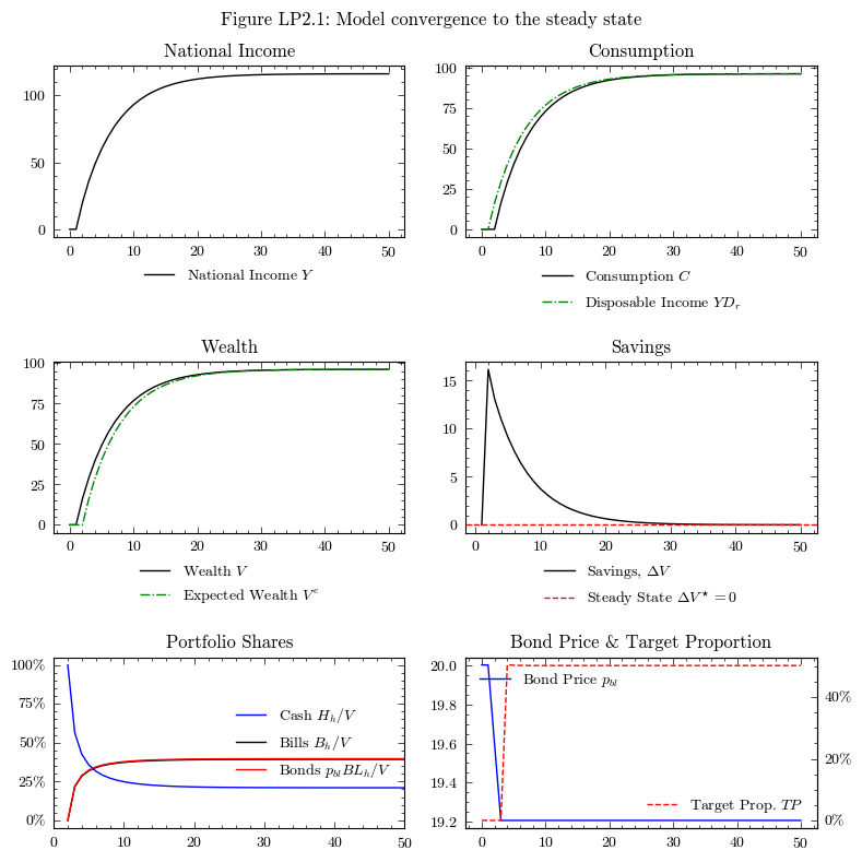
Convergence to the Steady State#
In the steady state of Model LP2, the target proportion \(TP\) stabilises within the band \([\text{bot}, \text{top}]\) and bond prices stop adjusting. Adaptive expectations converge to the actual bond price, so \(p_{bl}^e \to p_{bl}\), and capital gains vanish in the long run.
The convergence is slower than in LP because of the expectation feedback, but the long-run steady state is qualitatively similar.
dfo = output.loc[:50]

fig, axs = plt.subplots(ncols=2, nrows=3, figsize=(8, 8))

# National Income
axs[0, 0].plot(dfo.index, dfo['NationalIncome'], color='k', label=r'National Income $Y$')
axs[0, 0].legend(loc='upper center', bbox_to_anchor=(0.5, -0.1), frameon=False)
axs[0, 0].set_title('National Income')

# Consumption and Disposable Income
axs[0, 1].plot(dfo.index, dfo['ConsumptionHousehold'], color='k', label=r'Consumption $C$')
axs[0, 1].plot(dfo.index, dfo['DisposableIncome'], color='g', linestyle='-.', label=r'Disposable Income $YD_r$')
axs[0, 1].legend(loc='upper center', bbox_to_anchor=(0.5, -0.1), frameon=False)
axs[0, 1].set_title('Consumption')

# Wealth
axs[1, 0].plot(dfo.index, dfo['Wealth'], color='k', label=r'Wealth $V$')
axs[1, 0].plot(dfo.index, dfo['ExpectedWealth'], color='g', linestyle='-.', label=r'Expected Wealth $V^e$')
axs[1, 0].legend(loc='upper center', bbox_to_anchor=(0.5, -0.1), frameon=False)
axs[1, 0].set_title('Wealth')

# Savings
axs[1, 1].plot(dfo.index, dfo['Wealth'].diff(), color='k', label=r'Savings, $\Delta V$')
axs[1, 1].axhline(y=0, color='r', linestyle='--', label=r'Steady State $\Delta V^\star=0$')
axs[1, 1].legend(loc='upper center', bbox_to_anchor=(0.5, -0.1), frameon=False)
axs[1, 1].set_title('Savings')

# Portfolio Shares
cash_share = output['HouseholdCashStock'] / output['Wealth']
bill_share = output['HouseholdBillStock'] / output['Wealth']
bond_share = (output['HouseholdBondStock'].mul(output[('BondPrice','Macroeconomy')], axis=0)) / output['Wealth']

axs[2, 0].plot(output.index, cash_share, color='b', label='Cash $H_h/V$')
axs[2, 0].plot(output.index, bill_share, color='k', label='Bills $B_h/V$')
axs[2, 0].plot(output.index, bond_share, color='r', label='Bonds $p_{bl} BL_h/V$')
axs[2, 0].legend(loc='center right', frameon=False)
axs[2, 0].set_xlim(0, 50)
axs[2, 0].set_title('Portfolio Shares')
axs[2, 0].yaxis.set_major_formatter(PercentFormatter(1))

# Bond Price and Target Proportion
ax_bp = axs[2, 1]
ax_tp = ax_bp.twinx()
ax_bp.plot(dfo.index, dfo[('BondPrice', 'Macroeconomy')], color='b', label=r'Bond Price $p_{bl}$')
ax_tp.plot(dfo.index, dfo['TargetProportion'], color='r', linestyle='--', label=r'Target Prop. $TP$')
ax_bp.set_title('Bond Price & Target Proportion')
ax_bp.legend(loc='upper left', frameon=False)
ax_tp.legend(loc='lower right', frameon=False)
ax_tp.yaxis.set_major_formatter(PercentFormatter(1))

fig.suptitle('Figure LP2.1: Model convergence to the steady state')
plt.tight_layout()
plt.show()
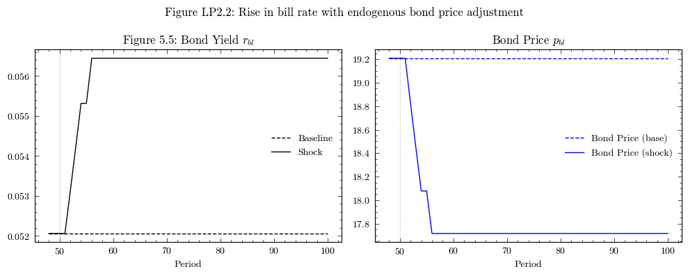
Perturbation 1: Rise in the Bill Rate (Section 5.8, first experiment)#
Following Section 5.8 of Godley and Lavoie [2006], we increase the interest rate on Treasury bills from 3% to 4%, but without changing the bond price exogenously (unlike Scenario 1 of LP). In LP2, the bond price adjusts endogenously through the target-proportion mechanism.
When \(r_b\) rises, bills become more attractive relative to bonds. Households shift their portfolio toward bills, which raises the target proportion \(TP\) above the upper threshold. The Treasury responds by allowing bond prices to rise until \(TP\) falls back into the target band. This is Figure 5.5 of Godley and Lavoie (2006).
scenarios = ScenariosGL06LP2(parameters=params)
sc1 = scenarios.get_scenario_index("Scenario.1: Rise in bill rate")
model1 = GL06LP2(parameters=params, scenarios=scenarios)
model1.simulate(scenario=sc1)
output_sc1 = model1.variables.to_pandas()
trigger = params["scenario_trigger"]
dfo = output_sc1.loc[trigger - 2:]
dfo_base = output.loc[trigger - 2:]

fig, axes = plt.subplots(1, 2, figsize=(10, 4))

# Figure 5.5: Bond yield
axes[0].plot(dfo_base.index, dfo_base['BondYield'], 'k--', label='Baseline')
axes[0].plot(dfo.index, dfo['BondYield'], 'k-', label='Shock')
axes[0].axvline(x=trigger, color='grey', linestyle=':', alpha=0.5)
axes[0].set_title('Figure 5.5: Bond Yield $r_{bl}$')
axes[0].set_xlabel('Period')
axes[0].legend(frameon=False)

# Bond Price
axes[1].plot(dfo_base.index, dfo_base[('BondPrice','Macroeconomy')], 'b--', label='Bond Price (base)')
axes[1].plot(dfo.index, dfo[('BondPrice','Macroeconomy')], 'b-', label='Bond Price (shock)')
axes[1].axvline(x=trigger, color='grey', linestyle=':', alpha=0.5)
axes[1].set_title('Bond Price $p_{bl}$')
axes[1].set_xlabel('Period')
axes[1].legend(frameon=False)

fig.suptitle('Figure LP2.2: Rise in bill rate with endogenous bond price adjustment')
plt.tight_layout()
plt.show()
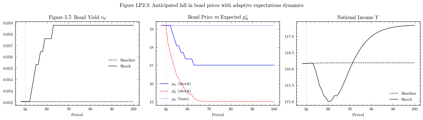
Perturbation 2: Anticipated Fall in Bond Prices (Section 5.8, second experiment)#
In this experiment, households form a one-period expectation of a fall in the bond price by 1 unit (via an ExpectedBondPriceShock of \(-1\)). The lower expected bond price reduces the expected return on bonds, causing households to demand fewer bonds and more bills and cash.
With adaptive expectations, this shock is only temporary — households gradually revise their expectations back toward the actual bond price. However, while the expectation shock persists, the portfolio reallocation depresses bond demand and, through the target-proportion mechanism, pushes bond prices lower. This is Figure 5.7 of Godley and Lavoie (2006).
sc2 = scenarios.get_scenario_index("Scenario.2: Expected bond price fall")
model2 = GL06LP2(parameters=params, scenarios=scenarios)
model2.simulate(scenario=sc2)
output_sc2 = model2.variables.to_pandas()
dfo2 = output_sc2.loc[trigger - 2:]

fig, axes = plt.subplots(1, 3, figsize=(14, 4))

# Figure 5.7: Bond yield
axes[0].plot(dfo_base.index, dfo_base['BondYield'], 'k--', label='Baseline')
axes[0].plot(dfo2.index, dfo2['BondYield'], 'k-', label='Shock')
axes[0].axvline(x=trigger, color='grey', linestyle=':', alpha=0.5)
axes[0].set_title('Figure 5.7: Bond Yield $r_{bl}$')
axes[0].set_xlabel('Period')
axes[0].legend(frameon=False)

# Bond Price vs Expected Bond Price
axes[1].plot(dfo2.index, dfo2[('BondPrice','Macroeconomy')], 'b-', label=r'$p_{bl}$ (shock)')
axes[1].plot(dfo2.index, dfo2['ExpectedBondPrice'], 'r--', label=r'$p_{bl}^e$ (shock)')
axes[1].plot(dfo_base.index, dfo_base[('BondPrice','Macroeconomy')], 'b:', label=r'$p_{bl}$ (base)')
axes[1].axvline(x=trigger, color='grey', linestyle=':', alpha=0.5)
axes[1].set_title(r'Bond Price vs Expected $p_{bl}^e$')
axes[1].set_xlabel('Period')
axes[1].legend(frameon=False)

# National Income
axes[2].plot(dfo_base.index, dfo_base['NationalIncome'], 'k--', label='Baseline')
axes[2].plot(dfo2.index, dfo2['NationalIncome'], 'k-', label='Shock')
axes[2].axvline(x=trigger, color='grey', linestyle=':', alpha=0.5)
axes[2].set_title('National Income $Y$')
axes[2].set_xlabel('Period')
axes[2].legend(frameon=False)

fig.suptitle('Figure LP2.3: Anticipated fall in bond prices with adaptive expectations dynamics')
plt.tight_layout()
plt.show()