Model SIMEX#

Model SIMEX is introduced in chapter 3 of Godley and Lavoie [2006] “Monetary Economics: An Integrated Approach to Credit, Money, Income, Production and Wealth” and represents the “simplest model with government money”. That is, this is a model with only outside money (from the government).

Module Contents#

As with all MacroStat models, SIMEX is divided into Variables, Parameters (fixed constants), Scenarios, and the Behavior (model initialization and steps). The module-level documentation, such as all variables/parameters/scenarios and their notation or the behavioral equations associated with each function of BehaviorSIM.py can be seen in:

Note

The remainder of this page gives an introduction to the model, notes on how it is implemented in MacroStat and then shows some of the model dynamics by replicating the relevant graphs of Godley and Lavoie (2006).

It is similar to Model SIM

Model Overview#

Behavioral Equations#

The SIMEX model is introduced in Chapter 3, and consists of the following 13 equations and 13 unknowns:

Consumption good supply equals demand

(1)#\[C_s(t) = C_d(t)\]

Governmend good supply equals demand

(2)#\[G_s(t) = G_d(t)\]

Tax supply equals demand

(3)#\[T_s(t) = T_d(t)\]

Labour supply equals demand

(4)#\[N_s(t) = N_d(t)\]

Disposable income is wage income minus taxes

(5)#\[YD(t) = W(t)\cdot N_s(t) - T_s(t)\]

Tax demand is a fixed proportion of wage income

(6)#\[T_d(t) = \theta\cdot W(t)\cdot N_s(t)\]

Consumption demand is a share of disposable income and deposits

(7)#\[C_d(t) = \alpha_1\cdot YD(t) + \alpha_2\cdot H_h(t-1)\]

The change in government stock of money is demand minus tax

(8)#\[\Delta H_s(t) = H_s(t) - H_s(t-1) = G_d(t) - T_d(t)\]

The change in household deposits is disposable income minus expenditure

(9)#\[\Delta H_h(t) = H_h(t) - H_h(t-1) = YD(t) - C_d(t)\]

Total national income is consumption of households and government

(10)#\[Y(t) = C_s(t) + G_s(t)\]

Labour Demand is national income over wages

(11)#\[N_d(t) = \frac{Y(t)}{W(t)}\]

Households’ demand for money is given by the excess of consumption demand over the current level of savings and expected income

(12)#\[\Delta H_d(t) = YD^e(t) - C_d(t)\]

Households’ expected disposable income is equal to their prior disposable income

(13)#\[YD^e(t) = YD(t-1)\]

With the redundant equation being

(14)#\[\Delta H_s(t) = \Delta H_h(t)\]

Transaction Flow Matrix#

Accounting Transaction Matrix for Model SIMEX#
	Household	Production	Government	Total
	Current	Current	Current
Consumption Supply	\(-C_s(t)\)	\(+C_s(t)\)		\(0\)
Government Supply		\(+G_s(t)\)	\(-G_s(t)\)	\(0\)
Tax Supply	\(-T_s(t)\)		\(+T_s(t)\)	\(0\)
Labour Income	\(+W(t)\cdot N_s(t)\)	\(-W(t)\cdot N_s(t)\)		\(0\)
Change in Money Stock	\(+\Delta H_h(t)\)		\(-\Delta H_s(t)\)	\(0\)
Total	\(0\)	\(0\)	\(0\)	\(0\)

Balance Sheet Matrix#

Balance Sheet for Model SIMEX#
	Household	Production	Government	Total
	Current	Current	Current
Money Stock	\(+H_h(t)\)		\(-H_s(t)\)	0

Implementation in MacroStat#

Transposing these eleven equations to the MacroStat framework, we consider that there are:

Three parameters (fixed constants): \(\alpha_1\), \(\alpha_2\), and \(\theta\) (see Parameters)
Two scenario variables : \(G_d(t)\) and \(W(t)\) (see Scenarios)
The remaining 16 tracked series are variables (see Variables)

Behavioral Modeling#

Unlike Model SIM, the determination of consumption demand based on expected disposable income means we do not need to rely on knowing ex ante the multiplier to resolve the model easily. Instead we can simply iterate forward. For a given period \(t\) we can solve the system by solving, in order:

Eq. (2) given the scenario variable
Eq. (13)
Consumption demand, given disposable income, Eq. (7)
Consumption supply, given demand, Eq. (1)
National income, Eq. (10)
Eq. (11) for labour demand
Eq. (4) for labour supply
Tax demand, given labour, Eq. (6)
Tax supply, given demand, Eq. (3)
Disposable income, given labour supply and tax demand, Eq. (5)
Government stock of money, Eq. (8)
Household demand for money, Eq. (12)
Household stock of deposits, Eq. (9)

This is implemented as such in the Behavior class.

Model Dynamics#

Preparatory Steps#

%load_ext autoreload
%autoreload 2

from matplotlib import pyplot as plt
from macrostat.models import get_model

plt.style.use("../../macrostat.mplstyle")

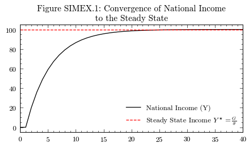
Convergence to the Steady State#

In Godley and Lavoie [2006] models are initialized with almost all of the variables set to zero. For model SIMEX the only non-zero item is that in period 0 the government demand is 20, i.e. the government creates 20 monetary units of demand. Thereafter the system converges to a steady state. We can see this by simulating the default parameters and checking that total national income is 100.

GL06SIMEX = get_model("GL06SIMEX")
model = GL06SIMEX()
model.simulate()
output = model.variables.to_pandas()

National Income#

steady_state_income = model.scenarios[(0,"GovernmentDemand")][0] / model.parameters["TaxRate"]

fig, axs = plt.subplots(1, 1, figsize=(5, 3))
axs.plot(output.index, output['NationalIncome'], color='k', label='National Income (Y)')
axs.axhline(y=steady_state_income, color='r', linestyle='--', label=r'Steady State Income $Y^\star=\frac{G}{\theta}$')
axs.legend(loc='lower right', frameon=False)
axs.set_xlim(0,40)
axs.set_title('Figure SIMEX.1: Convergence of National Income\nto the Steady State')
plt.tight_layout()
plt.show()

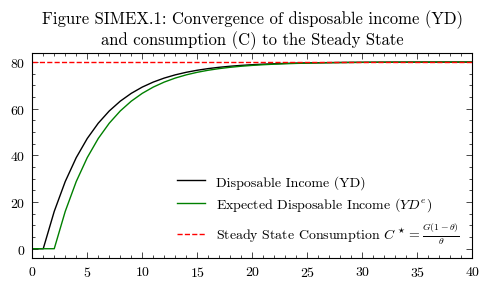
../../_images/b9f9000a15da7c00c1d00462b95f17056e90091de829989bc27d3a26afc7d59d.png

Disposable Income and Consumption#

Corresponding to Figure 3.2 “Disposable income and consumption starting from scratch”

steady_state_consumption= (model.scenarios[(0,"GovernmentDemand")][0] * (1-model.parameters["TaxRate"])) / model.parameters["TaxRate"]

fig, axs = plt.subplots(1, 1, figsize=(5, 3))
axs.plot(output.index, output['DisposableIncome'], color='k', label='Disposable Income (YD)')
axs.plot(output.index, output['ExpectedDisposableIncome'], color='g', label='Expected Disposable Income ($YD^e$)')
axs.axhline(y=steady_state_consumption, color='r', linestyle='--', label=r'Steady State Consumption $C^\star=\frac{G(1-\theta)}{\theta}$')
axs.legend(loc='lower right', frameon=False)
axs.set_xlim(0,40)
axs.set_title('Figure SIMEX.1: Convergence of disposable income (YD)\nand consumption (C) to the Steady State')
plt.tight_layout()
plt.show()

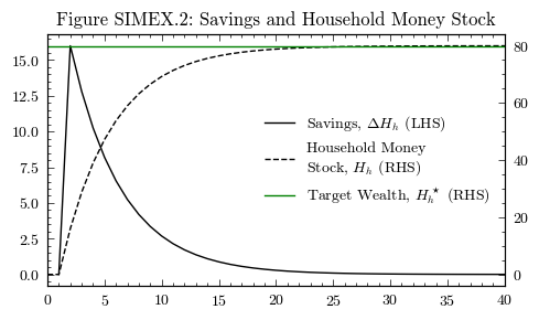
../../_images/8888b6270986f3e5f0028de216a7eb68ea1e057ca6f339441f9e69305e147c1e.png

Wealth and Savings#

Corresponding to Figure 3.3 “Wealth change and wealth level, starting from scratch (Table 3.4)”

alpha3 = (1-model.parameters["PropensityToConsumeSavings"]) / model.parameters["PropensityToConsumeIncome"]
steady_state_wealth = alpha3 * (model.scenarios[(0,"GovernmentDemand")][0] * (1-model.parameters["TaxRate"])) / model.parameters["TaxRate"]

fig, axs = plt.subplots(1, 1, figsize=(5, 3))
line1 = axs.plot(output.index, output['HouseholdMoneyStock'].diff(), color='k', label='Savings, $\Delta H_h$ (LHS)')
ax2 = axs.twinx()
line2 = ax2.plot(output.index, output['HouseholdMoneyStock'], color='k', linestyle='--', label='Household Money\nStock, $H_h$ (RHS)')
line3 = ax2.axhline(y=steady_state_wealth, color='g', label='Target Wealth, $H_h^\star$ (RHS)')
lines = line1 + line2 + [line3]
labels = [l.get_label() for l in lines]
axs.legend(lines, labels, loc='center right', frameon=False)
axs.set_xlim(0,40)
axs.set_title('Figure SIMEX.2: Savings and Household Money Stock')
plt.tight_layout()
plt.show()

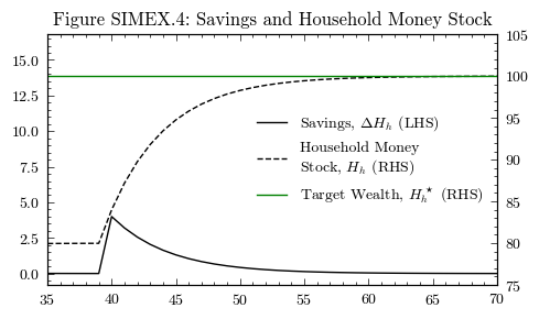
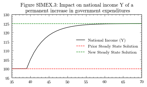
../../_images/3ed5dd4f1aa5f978edd1174afb482d7d408c777807a240ff74e4547eb0b22bda.png

Perturbations in the Steady State#

Following the convergence to the steady state, we can introduce a shock in government spending, increasing it by 5 units. Accordingly, the steady state given by \(Y^\star=\frac{G}{\theta}\) would shift to \(Y^\star=125\)

This kind of scenario can easily be implemented in the MacroStat version by adding a scenario:

Noting that we have convergence to the steady state at period 40, let us set this as the scenario trigger
We then need a new timeseries for the scenario, where \(G=25\) from the trigger period onwards

model.parameters["scenario_trigger"] = 40
model.scenarios.add_scenario(
    name="GovernmentDemandIncrease",
    timeseries={"GovernmentDemand":25}
)
model.simulate(scenario="GovernmentDemandIncrease")
output_government_demand_increase = model.variables.to_pandas()

National Income#

steady_state_income_new = model.scenarios[("GovernmentDemandIncrease","GovernmentDemand")][-1] / model.parameters["TaxRate"]

fig, axs = plt.subplots(1, 1, figsize=(5, 3))
axs.plot(output_government_demand_increase['NationalIncome'], color='k', label='National Income (Y)')
axs.axhline(y=steady_state_income, color='r', linestyle='--', label='Prior Steady State Solution')
axs.axhline(y=steady_state_income_new, color='g', linestyle='--', label='New Steady State Solution')
axs.legend(loc='center right', frameon=False)
axs.set_xlim(35,70)
axs.set_ylim(95,130)
axs.set_title('Figure SIMEX.3: Impact on national income Y of a\n permanent increase in government expenditures')
plt.tight_layout()
plt.show()

../../_images/8011b0b9869ca6bb3d3763b094f12cd699f23814feef7e1e5606344f7876f781.png

Consumption and Wealth#

steady_state_wealth_new = alpha3 * (model.scenarios[("GovernmentDemandIncrease","GovernmentDemand")][-1] * (1-model.parameters["TaxRate"])) / model.parameters["TaxRate"]

fig, axs = plt.subplots(1, 1, figsize=(5, 3))
line1 = axs.plot(output_government_demand_increase['HouseholdMoneyStock'].diff(), color='k', label='Savings, $\Delta H_h$ (LHS)')
ax2 = axs.twinx()
line2 = ax2.plot(output_government_demand_increase['HouseholdMoneyStock'], color='k', linestyle='--', label='Household Money\nStock, $H_h$ (RHS)')
line3 = ax2.axhline(y=steady_state_wealth_new, color='g', label='Target Wealth, $H_h^\star$ (RHS)')
lines = line1 + line2 + [line3]
labels = [l.get_label() for l in lines]
axs.legend(lines, labels, loc='center right', frameon=False)
axs.set_xlim(35,70)
ax2.set_ylim(75,105)
axs.set_title('Figure SIMEX.4: Savings and Household Money Stock')
plt.tight_layout()
plt.show()

../../_images/08b8b43ecdd12aeefcf5a0bbe48f8fb2f9d6534dddd46af600ca589ddfebfc24.png