ECO-3IO-PCEX (ECO3IOPC)

Model ECO-30IO-PCEX was introduced by Marco Veronese Passarella as a simple pedagogical environmentally extended stock-flow consistent (SFC) input-output (IO) model (see the source repository). This implementation by Karl Naumann-Woleske extends the model to use the expectation version of model PC.

Module Contents

As with all MacroStat models, ECOIOPC is divided into Variables, Parameters (fixed constants), Scenarios, and the Behavior (model initialization and steps). The module-level documentation, such as all variables/parameters/scenarios and their notation or the behavioral equations associated with each function of BehaviorECOIOPC.py can be seen in:

• Variables
• Parameters
  • Hyperparameters
  • Parameters
• Equations
  • Step Equations
• Scenarios

For the full model API please check the API Reference

Model Overview

The remainder of this page gives an introduction to the model, notes on how it is implemented in MacroStat and then shows some of the model dynamics using the default parameters.

Transaction Flow Matrix

Accounting Transaction Matrix for Model 3IO-PCEX

	Household	Government	CentralBank	CentralBank	IOSectors	Total
	Current	Current	Current	Capital	Current
Nominal Consumption Household	\(-p_c(t)c(t)\)				\(+p_c(t)c(t)\)	\(0\)
Nominal Consumption Government		\(-p_g(t) g(t)\)			\(+p_g(t) g(t)\)	\(0\)
National Income	\(+Y(t)\)				\(-Y(t)\)	\(0\)
Interest Earned On Bills Household	\(+r(t-1)\cdot B_h(t-1)\)	\(-r(t-1)\cdot B_h(t-1)\)				\(0\)
Central Bank Profits		\(+r(t-1)\cdot B_{CB}(t-1)\)	\(-r(t-1)\cdot B_{CB}(t-1)\)			\(0\)
Taxes	\(-T(t)\)	\(+T(t)\)				\(0\)
Change in Money Stock	\(+\Delta H_h(t)\)			\(-\Delta H_{s}(t)\)		\(0\)
Change in Bill Stock	\(+\Delta B_h(t)\)	\(-\Delta B_s(t)\)		\(+\Delta B_{CB}(t)\)		\(0\)
Total	\(0\)	\(0\)	\(0\)	\(0\)	\(0\)	\(0\)

Balance Sheet Matrix

Balance Sheet for Model 3IO-PCEX

	Household	Government	CentralBank	IOSectors	Total
	Current	Current	Capital	Current
Money Stock	\(+H_h(t)\)		\(-H_{s}(t)\)		0
Bill Stock	\(+B_h(t)\)	\(-B_s(t)\)	\(+B_{CB}(t)\)		0
Wealth	\(-V(t)\)	\(+V(t)\)			0

Model Dynamics

Preparatory Steps

%load_ext autoreload
%autoreload 2

import importlib
import logging
import sys

# Import the necessary libraries for plotting
from matplotlib import pyplot as plt
from matplotlib.ticker import PercentFormatter

# Import the MacroStat get_model function
from macrostat.models import get_model
from macrostat.causality import DocstringCausalityAnalyzer

# Custom matplotlib style for the documentation
plt.style.use("../../macrostat.mplstyle")
# We show the logging output in the notebook
importlib.reload(logging)
logging.basicConfig(stream=sys.stdout, level=logging.INFO)

Running the Simulation

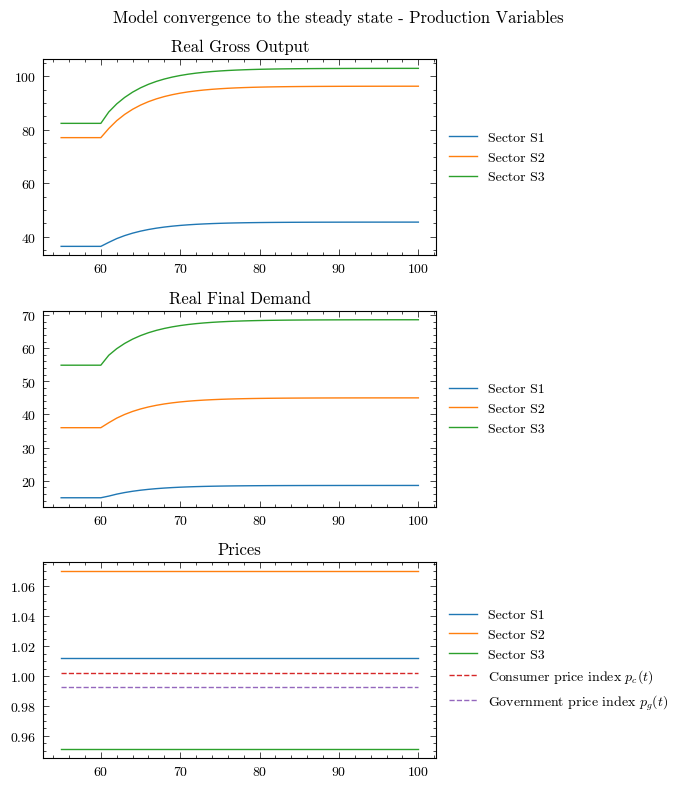
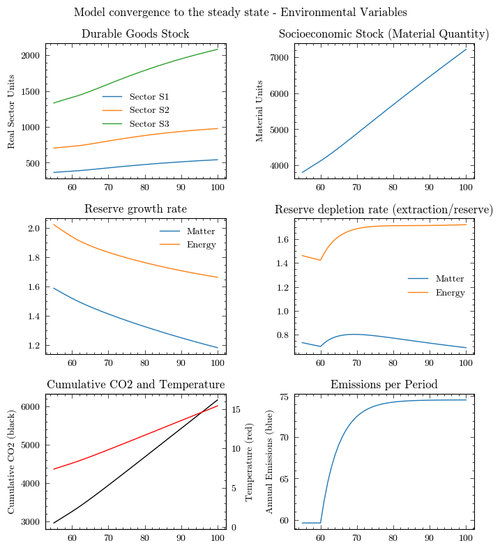
First, we can run the model without any shocks to see the convergence to the steady state.

ECO3IOPCClass = get_model("ECO3IOPC")
model = ECO3IOPCClass()
model.simulate()
output = model.variables.to_pandas()

Here we can also check that the variables are healthy, which means that the redundant equations hold and that all the assets and liabilities are positive. For model PC, the redundant equation is that the household money stock equals the central bank money stock.

Note

In numerical implementations, due to floating point precision it is unlikely that the redundant equation will hold exactly. Therefore, we check that the absolute percentage error is less than a given tolerance, in this case 1e-5. We use the absolute percentage error to appropriately scale the error for different magnitudes of the variables.

model.variables.check_health(tolerance=1e-5)

True

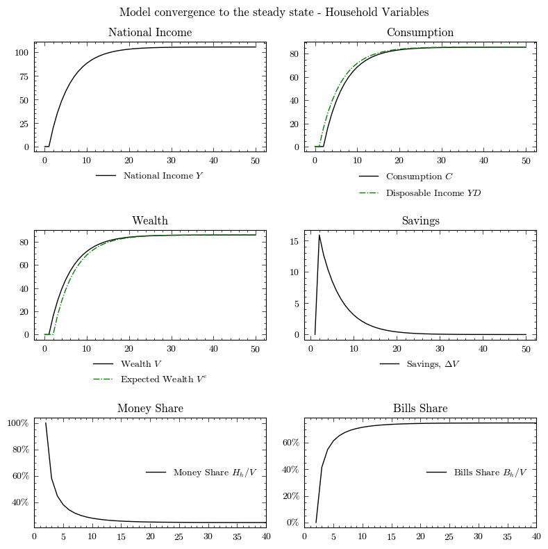
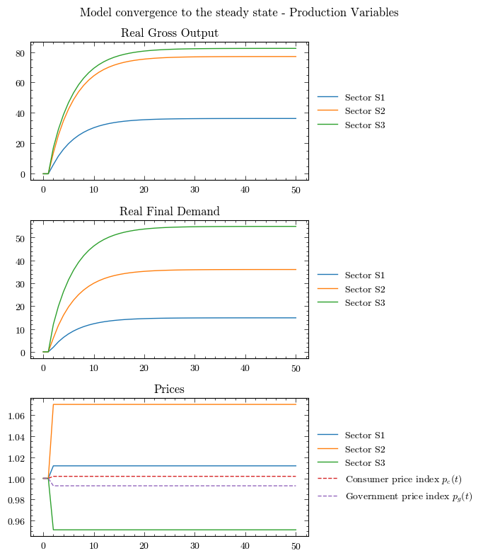
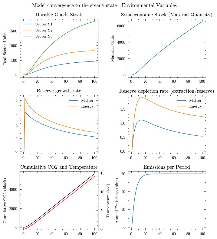
Convergence to the Steady State

Show code cell source

Hide code cell source

dfo = output.loc[:50]

fig, axs = plt.subplots(ncols=2, nrows=3, figsize=(8, 8))

# National Income and Consumption
axs[0,0].plot(dfo.index, dfo['NationalIncome'], color='k', label=r'National Income $Y$')
axs[0,0].legend(loc='upper center', bbox_to_anchor=(0.5, -0.1), frameon=False)
axs[0,0].set_title('National Income')
axs[0,1].plot(dfo.index, dfo['RealConsumptionHousehold'], color='k', label=r'Consumption $C$')
axs[0,1].plot(dfo.index, dfo['DisposableIncome'], color='g', linestyle='-.', label=r'Disposable Income $YD$')
axs[0,1].legend(loc='upper center', bbox_to_anchor=(0.5, -0.1), frameon=False)
axs[0,1].set_title('Consumption')

# Wealth and Savings
axs[1,0].plot(dfo.index, dfo['Wealth'], color='k', label=r'Wealth $V$')
axs[1,0].plot(dfo.index, dfo['ExpectedWealth'], color='g', linestyle='-.', label=r'Expected Wealth $V^e$')
axs[1,0].legend(loc='upper center', bbox_to_anchor=(0.5, -0.1), frameon=False)
axs[1,0].set_title('Wealth')
axs[1,1].plot(dfo.index, dfo['Wealth'].diff(), color='k', label=r'Savings, $\Delta V$')
axs[1,1].legend(loc='upper center', bbox_to_anchor=(0.5, -0.1), frameon=False)
axs[1,1].set_title('Savings')

# Money Share and Bills Share
axs[2,0].plot(dfo.index, dfo['HouseholdMoneyStock'] / dfo['Wealth'], color='k', linestyle='-', label='Money Share $H_h/V$')
axs[2,0].legend(loc='center right', frameon=False)
axs[2,0].set_xlim(0,40)
axs[2,0].set_title('Money Share')
axs[2,0].yaxis.set_major_formatter(PercentFormatter(1))

# Right panel - Bills share
axs[2,1].plot(dfo.index, dfo['HouseholdBillStock'] / dfo['Wealth'], color='k', linestyle='-', label='Bills Share $B_h/V$')
axs[2,1].legend(loc='center right', frameon=False)
axs[2,1].set_xlim(0,40)
axs[2,1].set_title('Bills Share')
axs[2,1].yaxis.set_major_formatter(PercentFormatter(1))


fig.suptitle('Model convergence to the steady state - Household Variables')
plt.tight_layout()
plt.show()

Show code cell source

Hide code cell source

dfo = output.loc[:50]

fig, axs = plt.subplots(ncols=1, nrows=3, figsize=(7, 8))

# National Income and Consumption
for s in dfo["RealGrossOutput"].columns:
    axs[0].plot(dfo.index, dfo['RealGrossOutput'][s], label=f"Sector {s}")
axs[0].set_title('Real Gross Output')

for s in dfo["RealFinalDemand"].columns:
    axs[1].plot(dfo.index, dfo['RealFinalDemand'][s], label=f"Sector {s}")
axs[1].set_title('Real Final Demand')

for s in dfo["Prices"].columns:
    axs[2].plot(dfo.index, dfo['Prices'][s], label=f"Sector {s}")
axs[2].plot(dfo.index, dfo["ConsumerPriceIndex"], linestyle="--", label=f"Consumer price index $p_c(t)$")
axs[2].plot(dfo.index, dfo["GovernmentPriceIndex"], linestyle="--", label=f"Government price index $p_g(t)$")
axs[2].set_title('Prices')

for ax in axs:
    ax.legend(loc='center left', bbox_to_anchor=(1.0, 0.5), frameon=False)


fig.suptitle('Model convergence to the steady state - Production Variables')
plt.tight_layout()
plt.show()

Show code cell source

Hide code cell source

dfo = output

fig, axs = plt.subplots(ncols=2, nrows=3, figsize=(7, 8))

axs[0,0].set_title("Durable Goods Stock")
axs[0,0].set_ylabel("Real Sector Units")
for s in dfo["DurableGoodsStock"].columns:
    axs[0,0].plot(dfo.index,dfo["DurableGoodsStock"][s], label=f"Sector {s}")

axs[0,1].set_title("Socioeconomic Stock (Material Quantity)")
axs[0,1].set_ylabel("Material Units")
axs[0,1].plot(dfo.index,dfo["SocioeconomicStock"])

axs[1,0].set_title("Reserve growth rate")
axs[1,0].plot(100 * dfo["ConversionMatterToReserves"] / dfo["MatterReserves"], label="Matter")
axs[1,0].plot(100 * dfo["ConversionEnergyToReserves"] / dfo["EnergyReserves"], label="Energy")

axs[1,1].set_title("Reserve depletion rate (extraction/reserve)")
axs[1,1].plot(100 * dfo["ExtractedMatter"] / dfo["MatterReserves"], label="Matter")
axs[1,1].plot(100 * dfo["EnergyRequiredForProduction"] / dfo["EnergyReserves"], label="Energy")

axs[2,0].set_title("Cumulative CO2 and Temperature")
axs[2,0].set_ylabel("Cumulative CO2 (black)")
axs[2,0].plot(dfo["CumulativeCO2"], color="black")
axs_alt = axs[2,0].twinx()
axs_alt.plot(dfo["Temperature"], color="red")
axs_alt.set_ylabel("Temperature (red)")
axs_alt.set_ylim(-0.25, 1.1 * dfo["Temperature"].max().iloc[0])

axs[2,1].set_title("Emissions per Period")
axs[2,1].plot(dfo["Emissions"])
axs[2,1].set_ylabel("Annual Emissions (blue)")

for ax in axs.flatten():
    ax.legend(frameon=False)

fig.suptitle('Model convergence to the steady state - Environmental Variables')
plt.tight_layout()
plt.show()

/tmp/ipykernel_646074/2998917229.py:35: UserWarning: No artists with labels found to put in legend.  Note that artists whose label start with an underscore are ignored when legend() is called with no argument.
  ax.legend(frameon=False)

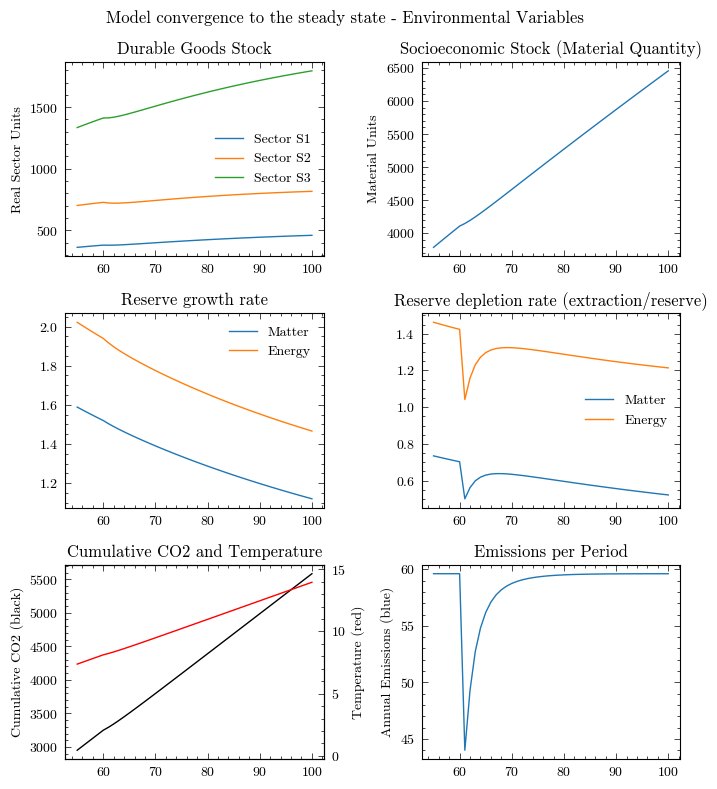
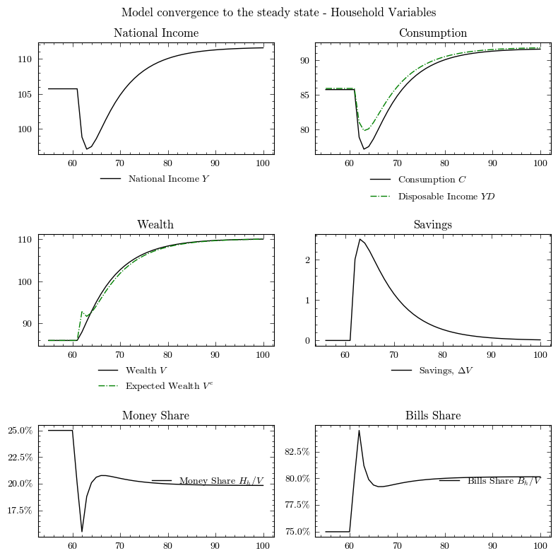
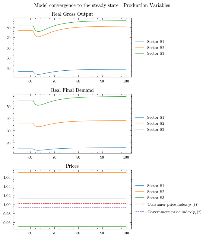
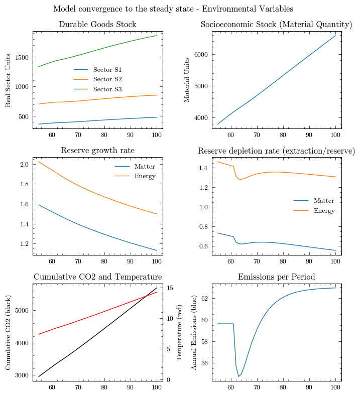
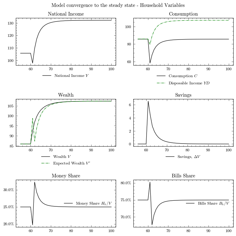
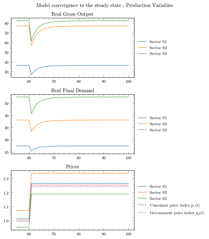
Perturbation 1: An increase of 100 points in the rate of interest on bills (\(r\))

Following the convergence to the steady state, we can study the effects of an increase in the rate on bills by 100bps

MacroStat is set up to easily handle these scenarios. Much like in prior models, we simply define a new scenario IncreaseInterestRate and set the new rate to be 100 points higher \(r=0.025+0.01\)

model.parameters["scenario_trigger"] = 60
model.scenarios.add_scenario(
    name="IncreaseInterestRate",
    timeseries={"InterestRate":0.025 + 0.01}
)
model.simulate(scenario="IncreaseInterestRate")
output_rate_increase = model.variables.to_pandas()

Now we can see how the model reacts to the shock.

The shock fires at scenario_trigger = 60. The plots below restrict the view to t >= 55 so the impulse window is visible.

Show code cell source

Hide code cell source

dfo = output_rate_increase.loc[55:]

fig, axs = plt.subplots(ncols=2, nrows=3, figsize=(8, 8))

# National Income and Consumption
axs[0,0].plot(dfo.index, dfo['NationalIncome'], color='k', label=r'National Income $Y$')
axs[0,0].legend(loc='upper center', bbox_to_anchor=(0.5, -0.1), frameon=False)
axs[0,0].set_title('National Income')
axs[0,1].plot(dfo.index, dfo['RealConsumptionHousehold'], color='k', label=r'Consumption $C$')
axs[0,1].plot(dfo.index, dfo['DisposableIncome'], color='g', linestyle='-.', label=r'Disposable Income $YD$')
axs[0,1].legend(loc='upper center', bbox_to_anchor=(0.5, -0.1), frameon=False)
axs[0,1].set_title('Consumption')

# Wealth and Savings
axs[1,0].plot(dfo.index, dfo['Wealth'], color='k', label=r'Wealth $V$')
axs[1,0].plot(dfo.index, dfo['ExpectedWealth'], color='g', linestyle='-.', label=r'Expected Wealth $V^e$')
axs[1,0].legend(loc='upper center', bbox_to_anchor=(0.5, -0.1), frameon=False)
axs[1,0].set_title('Wealth')
axs[1,1].plot(dfo.index, dfo['Wealth'].diff(), color='k', label=r'Savings, $\Delta V$')
axs[1,1].legend(loc='upper center', bbox_to_anchor=(0.5, -0.1), frameon=False)
axs[1,1].set_title('Savings')

# Money Share and Bills Share
axs[2,0].plot(dfo.index, dfo['HouseholdMoneyStock'] / dfo['Wealth'], color='k', linestyle='-', label='Money Share $H_h/V$')
axs[2,0].legend(loc='center right', frameon=False)
axs[2,0].set_title('Money Share')
axs[2,0].yaxis.set_major_formatter(PercentFormatter(1))

# Right panel - Bills share
axs[2,1].plot(dfo.index, dfo['HouseholdBillStock'] / dfo['Wealth'], color='k', linestyle='-', label='Bills Share $B_h/V$')
axs[2,1].legend(loc='center right', frameon=False)
axs[2,1].set_title('Bills Share')
axs[2,1].yaxis.set_major_formatter(PercentFormatter(1))


fig.suptitle('Model convergence to the steady state - Household Variables')
plt.tight_layout()
plt.show()

Show code cell source

Hide code cell source

dfo = output_rate_increase.loc[55:]

fig, axs = plt.subplots(ncols=1, nrows=3, figsize=(7, 8))

# National Income and Consumption
for s in dfo["RealGrossOutput"].columns:
    axs[0].plot(dfo.index, dfo['RealGrossOutput'][s], label=f"Sector {s}")
axs[0].set_title('Real Gross Output')

for s in dfo["RealFinalDemand"].columns:
    axs[1].plot(dfo.index, dfo['RealFinalDemand'][s], label=f"Sector {s}")
axs[1].set_title('Real Final Demand')

for s in dfo["Prices"].columns:
    axs[2].plot(dfo.index, dfo['Prices'][s], label=f"Sector {s}")
axs[2].plot(dfo.index, dfo["ConsumerPriceIndex"], linestyle="--", label=f"Consumer price index $p_c(t)$")
axs[2].plot(dfo.index, dfo["GovernmentPriceIndex"], linestyle="--", label=f"Government price index $p_g(t)$")
axs[2].set_title('Prices')

for ax in axs:
    ax.legend(loc='center left', bbox_to_anchor=(1.0, 0.5), frameon=False)


fig.suptitle('Model convergence to the steady state - Production Variables')
plt.tight_layout()
plt.show()

Show code cell source

Hide code cell source

fig, axs = plt.subplots(ncols=2, nrows=3, figsize=(7, 8))

axs[0,0].set_title("Durable Goods Stock")
axs[0,0].set_ylabel("Real Sector Units")
for s in dfo["DurableGoodsStock"].columns:
    axs[0,0].plot(dfo.index,dfo["DurableGoodsStock"][s], label=f"Sector {s}")

axs[0,1].set_title("Socioeconomic Stock (Material Quantity)")
axs[0,1].set_ylabel("Material Units")
axs[0,1].plot(dfo.index,dfo["SocioeconomicStock"])

axs[1,0].set_title("Reserve growth rate")
axs[1,0].plot(100 * dfo["ConversionMatterToReserves"] / dfo["MatterReserves"], label="Matter")
axs[1,0].plot(100 * dfo["ConversionEnergyToReserves"] / dfo["EnergyReserves"], label="Energy")

axs[1,1].set_title("Reserve depletion rate (extraction/reserve)")
axs[1,1].plot(100 * dfo["ExtractedMatter"] / dfo["MatterReserves"], label="Matter")
axs[1,1].plot(100 * dfo["EnergyRequiredForProduction"] / dfo["EnergyReserves"], label="Energy")

axs[2,0].set_title("Cumulative CO2 and Temperature")
axs[2,0].set_ylabel("Cumulative CO2 (black)")
axs[2,0].plot(dfo["CumulativeCO2"], color="black")
axs_alt = axs[2,0].twinx()
axs_alt.plot(dfo["Temperature"], color="red")
axs_alt.set_ylabel("Temperature (red)")
axs_alt.set_ylim(-0.25, 1.1 * dfo["Temperature"].max().iloc[0])

axs[2,1].set_title("Emissions per Period")
axs[2,1].plot(dfo["Emissions"])
axs[2,1].set_ylabel("Annual Emissions (blue)")

for ax in axs.flatten():
    ax.legend(frameon=False)

fig.suptitle('Model convergence to the steady state - Environmental Variables')
plt.tight_layout()
plt.show()

/tmp/ipykernel_646074/4078320462.py:33: UserWarning: No artists with labels found to put in legend.  Note that artists whose label start with an underscore are ignored when legend() is called with no argument.
  ax.legend(frameon=False)

Show code cell source

Hide code cell source

dfo = output

fig, axs = plt.subplots(ncols=2, nrows=3, figsize=(7, 8))

axs[0,0].set_title("Durable Goods Stock")
axs[0,0].set_ylabel("Real Sector Units")
for s in dfo["DurableGoodsStock"].columns:
    axs[0,0].plot(dfo.index,dfo["DurableGoodsStock"][s], label=f"Sector {s}")

axs[0,1].set_title("Socioeconomic Stock (Material Quantity)")
axs[0,1].set_ylabel("Material Units")
axs[0,1].plot(dfo.index,dfo["SocioeconomicStock"])

axs[1,0].set_title("Reserve growth rate")
axs[1,0].plot(100 * dfo["ConversionMatterToReserves"] / dfo["MatterReserves"], label="Matter")
axs[1,0].plot(100 * dfo["ConversionEnergyToReserves"] / dfo["EnergyReserves"], label="Energy")

axs[1,1].set_title("Reserve depletion rate (extraction/reserve)")
axs[1,1].plot(100 * dfo["ExtractedMatter"] / dfo["MatterReserves"], label="Matter")
axs[1,1].plot(100 * dfo["EnergyRequiredForProduction"] / dfo["EnergyReserves"], label="Energy")

axs[2,0].set_title("Cumulative CO2 and Temperature")
axs[2,0].set_ylabel("Cumulative CO2 (black)")
axs[2,0].plot(dfo["CumulativeCO2"], color="black")
axs_alt = axs[2,0].twinx()
axs_alt.plot(dfo["Temperature"], color="red")
axs_alt.set_ylabel("Temperature (red)")
axs_alt.set_ylim(-0.25, 1.1 * dfo["Temperature"].max().iloc[0])

axs[2,1].set_title("Emissions per Period")
axs[2,1].plot(dfo["Emissions"])
axs[2,1].set_ylabel("Annual Emissions (blue)")

for ax in axs.flatten():
    ax.legend(frameon=False)

fig.suptitle('Model convergence to the steady state - Environmental Variables')
plt.tight_layout()
plt.show()

/tmp/ipykernel_646074/2998917229.py:35: UserWarning: No artists with labels found to put in legend.  Note that artists whose label start with an underscore are ignored when legend() is called with no argument.
  ax.legend(frameon=False)

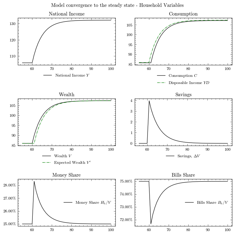
Perturbation 2: An increate in government spending

model.parameters["scenario_trigger"] = 60
model.scenarios.add_scenario(
    name="GovSpending",
    timeseries={"GovernmentDemand":25}
)
model.simulate(scenario="GovSpending")
output= model.variables.to_pandas()
dfo = output.loc[55:]

Show code cell source

Hide code cell source

fig, axs = plt.subplots(ncols=2, nrows=3, figsize=(8, 8))

# National Income and Consumption
axs[0,0].plot(dfo.index, dfo['NationalIncome'], color='k', label=r'National Income $Y$')
axs[0,0].legend(loc='upper center', bbox_to_anchor=(0.5, -0.1), frameon=False)
axs[0,0].set_title('National Income')
axs[0,1].plot(dfo.index, dfo['RealConsumptionHousehold'], color='k', label=r'Consumption $C$')
axs[0,1].plot(dfo.index, dfo['DisposableIncome'], color='g', linestyle='-.', label=r'Disposable Income $YD$')
axs[0,1].legend(loc='upper center', bbox_to_anchor=(0.5, -0.1), frameon=False)
axs[0,1].set_title('Consumption')

# Wealth and Savings
axs[1,0].plot(dfo.index, dfo['Wealth'], color='k', label=r'Wealth $V$')
axs[1,0].plot(dfo.index, dfo['ExpectedWealth'], color='g', linestyle='-.', label=r'Expected Wealth $V^e$')
axs[1,0].legend(loc='upper center', bbox_to_anchor=(0.5, -0.1), frameon=False)
axs[1,0].set_title('Wealth')
axs[1,1].plot(dfo.index, dfo['Wealth'].diff(), color='k', label=r'Savings, $\Delta V$')
axs[1,1].legend(loc='upper center', bbox_to_anchor=(0.5, -0.1), frameon=False)
axs[1,1].set_title('Savings')

# Money Share and Bills Share
axs[2,0].plot(dfo.index, dfo['HouseholdMoneyStock'] / dfo['Wealth'], color='k', linestyle='-', label='Money Share $H_h/V$')
axs[2,0].legend(loc='center right', frameon=False)
axs[2,0].set_title('Money Share')
axs[2,0].yaxis.set_major_formatter(PercentFormatter(1))

# Right panel - Bills share
axs[2,1].plot(dfo.index, dfo['HouseholdBillStock'] / dfo['Wealth'], color='k', linestyle='-', label='Bills Share $B_h/V$')
axs[2,1].legend(loc='center right', frameon=False)
axs[2,1].set_title('Bills Share')
axs[2,1].yaxis.set_major_formatter(PercentFormatter(1))


fig.suptitle('Model convergence to the steady state - Household Variables')
plt.tight_layout()
plt.show()

Show code cell source

Hide code cell source

fig, axs = plt.subplots(ncols=1, nrows=3, figsize=(7, 8))

# National Income and Consumption
for s in dfo["RealGrossOutput"].columns:
    axs[0].plot(dfo.index, dfo['RealGrossOutput'][s], label=f"Sector {s}")
axs[0].set_title('Real Gross Output')

for s in dfo["RealFinalDemand"].columns:
    axs[1].plot(dfo.index, dfo['RealFinalDemand'][s], label=f"Sector {s}")
axs[1].set_title('Real Final Demand')

for s in dfo["Prices"].columns:
    axs[2].plot(dfo.index, dfo['Prices'][s], label=f"Sector {s}")
axs[2].plot(dfo.index, dfo["ConsumerPriceIndex"], linestyle="--", label=f"Consumer price index $p_c(t)$")
axs[2].plot(dfo.index, dfo["GovernmentPriceIndex"], linestyle="--", label=f"Government price index $p_g(t)$")
axs[2].set_title('Prices')

for ax in axs:
    ax.legend(loc='center left', bbox_to_anchor=(1.0, 0.5), frameon=False)


fig.suptitle('Model convergence to the steady state - Production Variables')
plt.tight_layout()
plt.show()

Show code cell source

Hide code cell source

fig, axs = plt.subplots(ncols=2, nrows=3, figsize=(7, 8))

axs[0,0].set_title("Durable Goods Stock")
axs[0,0].set_ylabel("Real Sector Units")
for s in dfo["DurableGoodsStock"].columns:
    axs[0,0].plot(dfo.index,dfo["DurableGoodsStock"][s], label=f"Sector {s}")

axs[0,1].set_title("Socioeconomic Stock (Material Quantity)")
axs[0,1].set_ylabel("Material Units")
axs[0,1].plot(dfo.index,dfo["SocioeconomicStock"])

axs[1,0].set_title("Reserve growth rate")
axs[1,0].plot(100 * dfo["ConversionMatterToReserves"] / dfo["MatterReserves"], label="Matter")
axs[1,0].plot(100 * dfo["ConversionEnergyToReserves"] / dfo["EnergyReserves"], label="Energy")

axs[1,1].set_title("Reserve depletion rate (extraction/reserve)")
axs[1,1].plot(100 * dfo["ExtractedMatter"] / dfo["MatterReserves"], label="Matter")
axs[1,1].plot(100 * dfo["EnergyRequiredForProduction"] / dfo["EnergyReserves"], label="Energy")

axs[2,0].set_title("Cumulative CO2 and Temperature")
axs[2,0].set_ylabel("Cumulative CO2 (black)")
axs[2,0].plot(dfo["CumulativeCO2"], color="black")
axs_alt = axs[2,0].twinx()
axs_alt.plot(dfo["Temperature"], color="red")
axs_alt.set_ylabel("Temperature (red)")
axs_alt.set_ylim(-0.25, 1.1 * dfo["Temperature"].max().iloc[0])

axs[2,1].set_title("Emissions per Period")
axs[2,1].plot(dfo["Emissions"])
axs[2,1].set_ylabel("Annual Emissions (blue)")

for ax in axs.flatten():
    ax.legend(frameon=False)

fig.suptitle('Model convergence to the steady state - Environmental Variables')
plt.tight_layout()
plt.show()

/tmp/ipykernel_646074/4078320462.py:33: UserWarning: No artists with labels found to put in legend.  Note that artists whose label start with an underscore are ignored when legend() is called with no argument.
  ax.legend(frameon=False)

Perturbation 3: An increase in the wage rate

model.parameters["scenario_trigger"] = 60
model.scenarios.add_scenario(
    name="WageRate",
    timeseries={"WageRate":0.5}
)
model.simulate(scenario="WageRate")
output_wage_rate_increase = model.variables.to_pandas()
dfo = output_wage_rate_increase.loc[55:]

Show code cell source

Hide code cell source

fig, axs = plt.subplots(ncols=2, nrows=3, figsize=(8, 8))

# National Income and Consumption
axs[0,0].plot(dfo.index, dfo['NationalIncome'], color='k', label=r'National Income $Y$')
axs[0,0].legend(loc='upper center', bbox_to_anchor=(0.5, -0.1), frameon=False)
axs[0,0].set_title('National Income')
axs[0,1].plot(dfo.index, dfo['RealConsumptionHousehold'], color='k', label=r'Consumption $C$')
axs[0,1].plot(dfo.index, dfo['DisposableIncome'], color='g', linestyle='-.', label=r'Disposable Income $YD$')
axs[0,1].legend(loc='upper center', bbox_to_anchor=(0.5, -0.1), frameon=False)
axs[0,1].set_title('Consumption')

# Wealth and Savings
axs[1,0].plot(dfo.index, dfo['Wealth'], color='k', label=r'Wealth $V$')
axs[1,0].plot(dfo.index, dfo['ExpectedWealth'], color='g', linestyle='-.', label=r'Expected Wealth $V^e$')
axs[1,0].legend(loc='upper center', bbox_to_anchor=(0.5, -0.1), frameon=False)
axs[1,0].set_title('Wealth')
axs[1,1].plot(dfo.index, dfo['Wealth'].diff(), color='k', label=r'Savings, $\Delta V$')
axs[1,1].legend(loc='upper center', bbox_to_anchor=(0.5, -0.1), frameon=False)
axs[1,1].set_title('Savings')

# Money Share and Bills Share
axs[2,0].plot(dfo.index, dfo['HouseholdMoneyStock'] / dfo['Wealth'], color='k', linestyle='-', label='Money Share $H_h/V$')
axs[2,0].legend(loc='center right', frameon=False)
axs[2,0].set_title('Money Share')
axs[2,0].yaxis.set_major_formatter(PercentFormatter(1))

# Right panel - Bills share
axs[2,1].plot(dfo.index, dfo['HouseholdBillStock'] / dfo['Wealth'], color='k', linestyle='-', label='Bills Share $B_h/V$')
axs[2,1].legend(loc='center right', frameon=False)
axs[2,1].set_title('Bills Share')
axs[2,1].yaxis.set_major_formatter(PercentFormatter(1))


fig.suptitle('Model convergence to the steady state - Household Variables')
plt.tight_layout()
plt.show()

Show code cell source

Hide code cell source

fig, axs = plt.subplots(ncols=1, nrows=3, figsize=(7, 8))

# National Income and Consumption
for s in dfo["RealGrossOutput"].columns:
    axs[0].plot(dfo.index, dfo['RealGrossOutput'][s], label=f"Sector {s}")
axs[0].set_title('Real Gross Output')

for s in dfo["RealFinalDemand"].columns:
    axs[1].plot(dfo.index, dfo['RealFinalDemand'][s], label=f"Sector {s}")
axs[1].set_title('Real Final Demand')

for s in dfo["Prices"].columns:
    axs[2].plot(dfo.index, dfo['Prices'][s], label=f"Sector {s}")
axs[2].plot(dfo.index, dfo["ConsumerPriceIndex"], linestyle="--", label=f"Consumer price index $p_c(t)$")
axs[2].plot(dfo.index, dfo["GovernmentPriceIndex"], linestyle="--", label=f"Government price index $p_g(t)$")
axs[2].set_title('Prices')

for ax in axs:
    ax.legend(loc='center left', bbox_to_anchor=(1.0, 0.5), frameon=False)


fig.suptitle('Model convergence to the steady state - Production Variables')
plt.tight_layout()
plt.show()

Show code cell source

Hide code cell source

fig, axs = plt.subplots(ncols=2, nrows=3, figsize=(7, 8))

axs[0,0].set_title("Durable Goods Stock")
axs[0,0].set_ylabel("Real Sector Units")
for s in dfo["DurableGoodsStock"].columns:
    axs[0,0].plot(dfo.index,dfo["DurableGoodsStock"][s], label=f"Sector {s}")

axs[0,1].set_title("Socioeconomic Stock (Material Quantity)")
axs[0,1].set_ylabel("Material Units")
axs[0,1].plot(dfo.index,dfo["SocioeconomicStock"])

axs[1,0].set_title("Reserve growth rate")
axs[1,0].plot(100 * dfo["ConversionMatterToReserves"] / dfo["MatterReserves"], label="Matter")
axs[1,0].plot(100 * dfo["ConversionEnergyToReserves"] / dfo["EnergyReserves"], label="Energy")

axs[1,1].set_title("Reserve depletion rate (extraction/reserve)")
axs[1,1].plot(100 * dfo["ExtractedMatter"] / dfo["MatterReserves"], label="Matter")
axs[1,1].plot(100 * dfo["EnergyRequiredForProduction"] / dfo["EnergyReserves"], label="Energy")

axs[2,0].set_title("Cumulative CO2 and Temperature")
axs[2,0].set_ylabel("Cumulative CO2 (black)")
axs[2,0].plot(dfo["CumulativeCO2"], color="black")
axs_alt = axs[2,0].twinx()
axs_alt.plot(dfo["Temperature"], color="red")
axs_alt.set_ylabel("Temperature (red)")
axs_alt.set_ylim(-0.25, 1.1 * dfo["Temperature"].max().iloc[0])

axs[2,1].set_title("Emissions per Period")
axs[2,1].plot(dfo["Emissions"])
axs[2,1].set_ylabel("Annual Emissions (blue)")

for ax in axs.flatten():
    ax.legend(frameon=False)

fig.suptitle('Model convergence to the steady state - Environmental Variables')
plt.tight_layout()
plt.show()

/tmp/ipykernel_646074/4078320462.py:33: UserWarning: No artists with labels found to put in legend.  Note that artists whose label start with an underscore are ignored when legend() is called with no argument.
  ax.legend(frameon=False)