Model PCEX2#

Model PCEX is introduced in chapter 4 of Godley and Lavoie [2006] “Monetary Economics: An Integrated Approach to Credit, Money, Income, Production and Wealth”. In its setup, the model has the same transactions and balance sheet as Model PC (see here), but features expectations on disposable income and wealth.

Module Contents#

As with all MacroStat models, PCEX is divided into Variables, Parameters (fixed constants), Scenarios, and the Behavior (model initialization and steps). The module-level documentation, such as all variables/parameters/scenarios and their notation or the behavioral equations associated with each function of BehaviorPCEX.py can be seen in:

The remainder of this page gives an introduction to the model, notes on how it is implemented in MacroStat and then shows some of the model dynamics by replicating the relevant graphs of Godley and Lavoie (2006).

Model Overview#

Behavioral Equations#

Model PCEX2 is an extension of Model PCEX with only one change in equations, namely that we replace the fixed propensity to consume out of income, \(\alpha_1\) with is transformed to

(1)#\[\alpha_1(t) = \alpha_{10} + \iota r(t-1)\]

Accordingly, see PCEX for a guide on the remaining equations, or see the behavior documentation.

Transaction Flow Matrix#

Accounting Transaction Matrix for Model PCEX2#
	Household	Production	Government	CentralBank	CentralBank	Total
	Current	Current	Current	Current	Capital
Consumption Household	\(-C(t)\)	\(+C(t)\)				\(0\)
Consumption Government		\(+G(t)\)	\(-G(t)\)			\(0\)
National Income	\(+Y(t)\)	\(-Y(t)\)				\(0\)
Interest Earned On Bills Household	\(+r(t-1)\cdot B_h(t-1)\)		\(-r(t-1)\cdot B_h(t-1)\)			\(0\)
Central Bank Profits			\(+r(t-1)\cdot B_{CB}(t-1)\)	\(-r(t-1)\cdot B_{CB}(t-1)\)		\(0\)
Taxes	\(-T(t)\)		\(+T(t)\)			\(0\)
Change in Money Stock	\(+\Delta H_h(t)\)				\(-\Delta H_{s}(t)\)	\(0\)
Change in Bill Stock	\(+\Delta B_h(t)\)		\(-\Delta B_s(t)\)		\(+\Delta B_{CB}(t)\)	\(0\)
Total	\(0\)	\(0\)	\(0\)	\(0\)	\(0\)	\(0\)

Balance Sheet Matrix#

Balance Sheet for Model PCEX2#
	Household	Production	Government	CentralBank	Total
	Current	Current	Current	Capital
Money Stock	\(+H_h(t)\)			\(-H_{s}(t)\)	0
Bill Stock	\(+B_h(t)\)		\(-B_s(t)\)	\(+B_{CB}(t)\)	0
Wealth	\(-V(t)\)		\(+V(t)\)		0

Implementation in MacroStat#

Transposing these eleven equations to the MacroStat framework, we consider that there are:

Four parameters (fixed constants): \(\alpha_{10}\), \(\iota\), \(\alpha_2\), and \(\theta\) (see Parameters)
Two scenario variables : \(G_d(t)\) and \(W(t)\) (see Scenarios)
The remaining tracked series are variables (see Variables)

Model Dynamics#

Preparatory Steps#

%load_ext autoreload
%autoreload 2

import importlib
import logging
import sys

# Import the necessary libraries for plotting
from matplotlib import pyplot as plt
from matplotlib.ticker import PercentFormatter

# Import the MacroStat get_model function
from macrostat.models import get_model

# Custom matplotlib style for the documentation
plt.style.use("../../macrostat.mplstyle")
# We show the logging output in the notebook
importlib.reload(logging)
logging.basicConfig(stream=sys.stdout, level=logging.INFO)

Running the Simulation#

First, we can run the model without any shocks to see the convergence to the steady state.

GL06PCEX2Class = get_model("GL06PCEX2")
model = GL06PCEX2Class()
model.simulate()
output = model.variables.to_pandas()

INFO:root:Starting simulation. Scenario: 0

Here we can also check that the variables are healthy, which means that the redundant equations hold and that all the assets and liabilities are positive. For model PC, the redundant equation is that the household money stock equals the central bank money stock.

Note

In numerical implementations, due to floating point precision it is unlikely that the redundant equation will hold exactly. Therefore, we check that the absolute percentage error is less than a given tolerance, in this case 1e-5. We use the absolute percentage error to appropriately scale the error for different magnitudes of the variables.

model.variables.check_health(tolerance=1e-5)

True

An overview of the first 10 steps of the model

df=model.variables.to_pandas()
df.head(10).T

	2	3	4	5	6	7	8	9
ConsumptionHousehold	0.000	16.000000	28.799999	39.279999	47.855999	54.874001	60.617043	65.316742
ConsumptionGovernment	20.000	20.000000	20.000000	20.000000	20.000000	20.000000	20.000000	20.000000
NationalIncome	20.000	36.000000	48.799999	59.279999	67.856003	74.874001	80.617043	85.316742
InterestEarnedOnBillsHousehold	0.000	0.000000	0.300000	0.540000	0.736500	0.897300	1.028888	1.136570
CentralBankProfits	0.000	0.400000	0.420000	0.442000	0.459900	0.474550	0.486538	0.496349
Taxes	4.000	7.200000	9.820000	11.964000	13.718501	15.154261	16.329185	17.290663
HouseholdMoneyStock	16.000	16.799999	17.680004	18.396004	18.981998	19.461540	19.853958	20.175087
CentralBankMoneyStock	16.000	16.800003	17.680002	18.396004	18.981991	19.461536	19.853958	20.175095
HouseholdBillStock	0.000	12.000000	21.599998	29.459999	35.892006	41.155502	45.462784	48.987556
GovernmentBillStock	16.000	28.800001	39.279999	47.856003	54.873997	60.617039	65.316742	69.162651
CentralBankBillStock	16.000	16.800001	17.680000	18.396004	18.981991	19.461536	19.853958	20.175095
Wealth	16.000	28.799999	39.280003	47.856003	54.874004	60.617043	65.316742	69.162643
InterestRate	0.025	0.025000	0.025000	0.025000	0.025000	0.025000	0.025000	0.025000
DisposableIncome	16.000	28.799999	39.279999	47.855999	54.874001	60.617043	65.316742	69.162643
ExpectedDisposableIncome	0.000	16.000000	28.799999	39.279999	47.855999	54.874001	60.617043	65.316742
ExpectedWealth	0.000	16.000000	28.799999	39.279999	47.856007	54.874001	60.617043	65.316742
HouseholdBillDemand	0.000	12.000000	21.599998	29.459999	35.892006	41.155502	45.462784	48.987556

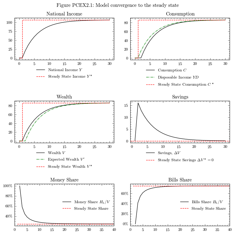
Convergence to the Steady State#

The steady state for Model PCEX is equivalent to model PC, it just has delays in reathing the steady state. In Godley and Lavoie [2006] models are initialized with almost all of the variables set to zero. For model PCEX the only non-zero item is that in period 0 the government demand is 20, i.e. the government creates 20 monetary units of demand.

To aid in our graphing, we can calculate the steady state solutions for the variables following the derivations in Section 4.5 of Godley and Lavoie Godley and Lavoie [2006]:

\[\begin{split}\begin{align} G^\star(t) &= G(t)\\ r^\star(t) &= r(t)\\ \alpha_3 &= \frac{1-(\alpha_{10} - \iota r^\star(t))}{\alpha_2}\\ YD^\star(t) = YD^{e\star}(t) &= \frac{G^\star(t)}{\frac{\theta}{1-\theta} - r^\star(t)\cdot\left(\left(\lambda_0 + \lambda_1 r^\star(t) \right)\alpha_3 - \lambda_2\right)}\\ C^\star(t) &= YD^\star(t)\\ Y^\star(t) &= C^\star(t) + G^\star(t)\\ V^\star(t) = V^{e\star}(t) &= \alpha_3 YD^\star(t)\\ B_d^\star(t) = B_h^\star(t) &= \left(\left(\lambda_0 + \lambda_1 r^\star(t) \right)\alpha_3 - \lambda_2\right)\cdot YD^\star(t)\\ T^\star(t) &= \theta\cdot \left(Y^\star(t) + r^\star(t) B_h^\star(t)\right)\\ H_h^\star(t) &= V^{e\star}(t) - B_h^\star(t)\\ B_s^\star(t) &= \frac{r^\star(t) B_{CB}^\star(t) + T^\star(t) - G^\star(t)}{r^\star(t)}\\ B_{CB}^\star(t) &= B_s^\star(t) - B_h^\star(t)\\ H_s^\star(t) &= H_{s}(t-1) + (B_{CB}(t) - B_{CB}(t-1)) \end{align}\end{split}\]

In macrostat, this solution has been implemented in the compute_theoretical_steady_state() function. We compute this now for scenario=0, which is the case without any shocks and constant government demand \(G\) and interest rates \(r\).

model.compute_theoretical_steady_state(scenario=0)
steadystate = model.variables.to_pandas()

INFO:root:Computing theoretical steady state. Scenario: 0

Show code cell source

Hide code cell source

dfo = output.loc[:30]
dfs = steadystate.loc[:30]

fig, axs = plt.subplots(ncols=2, nrows=3, figsize=(8, 8))

# National Income and Consumption
axs[0,0].plot(dfo.index, dfo['NationalIncome'], color='k', label=r'National Income $Y$')
axs[0,0].step(x=dfs.index,y=dfs["NationalIncome"], color='r', linestyle='--', label=r'Steady State Income $Y^\star$')
axs[0,0].legend(loc='upper center', bbox_to_anchor=(0.5, -0.1), frameon=False)
axs[0,0].set_title('National Income')
axs[0,1].plot(dfo.index, dfo['ConsumptionHousehold'], color='k', label=r'Consumption $C$')
axs[0,1].plot(dfo.index, dfo['DisposableIncome'], color='g', linestyle='-.', label=r'Disposable Income $YD$')
axs[0,1].step(x=dfs.index,y=dfs["ConsumptionHousehold"], color='r', linestyle='--', label=r'Steady State Consumption $C^\star$')
axs[0,1].legend(loc='upper center', bbox_to_anchor=(0.5, -0.1), frameon=False)
axs[0,1].set_title('Consumption')

# Wealth and Savings
axs[1,0].plot(dfo.index, dfo['Wealth'], color='k', label=r'Wealth $V$')
axs[1,0].plot(dfo.index, dfo['ExpectedWealth'], color='g', linestyle='-.', label=r'Expected Wealth $V^e$')
axs[1,0].step(x=dfs.index,y=dfs["Wealth"], color='r', linestyle='--', label=r'Steady State Wealth $V^\star$')
axs[1,0].legend(loc='upper center', bbox_to_anchor=(0.5, -0.1), frameon=False)
axs[1,0].set_title('Wealth')
axs[1,1].plot(dfo.index, dfo['Wealth'].diff(), color='k', label=r'Savings, $\Delta V$')
axs[1,1].axhline(y=0, color='r', linestyle='--', label=r'Steady State Savings $\Delta V^\star=0$')
axs[1,1].legend(loc='upper center', bbox_to_anchor=(0.5, -0.1), frameon=False)
axs[1,1].set_title('Savings')

# Money Share and Bills Share
share_bills = steadystate['HouseholdBillStock'] / steadystate['Wealth']
axs[2,0].plot(output.index, output['HouseholdMoneyStock'] / output['Wealth'], color='k', linestyle='-', label='Money Share $H_h/V$')
axs[2,0].step(x=share_bills.index,y=1-share_bills, color='r', linestyle='--', label='Steady State Share')
axs[2,0].legend(loc='center right', frameon=False)
axs[2,0].set_xlim(0,40)
axs[2,0].set_title('Money Share')
axs[2,0].yaxis.set_major_formatter(PercentFormatter(1))

# Right panel - Bills share
axs[2,1].plot(output.index, output['HouseholdBillStock'] / output['Wealth'], color='k', linestyle='-', label='Bills Share $B_h/V$')
axs[2,1].step(x=share_bills.index,y=share_bills, color='r', linestyle='--', label='Steady State Share')
axs[2,1].legend(loc='center right', frameon=False)
axs[2,1].set_xlim(0,40)
axs[2,1].set_title('Bills Share')
axs[2,1].yaxis.set_major_formatter(PercentFormatter(1))


fig.suptitle('Figure PCEX2.1: Model convergence to the steady state')
plt.tight_layout()
plt.show()

../../_images/b476c24815f31bfbed074381d481b767cd7bbed24ede9d2971c93bed4d156a24.png

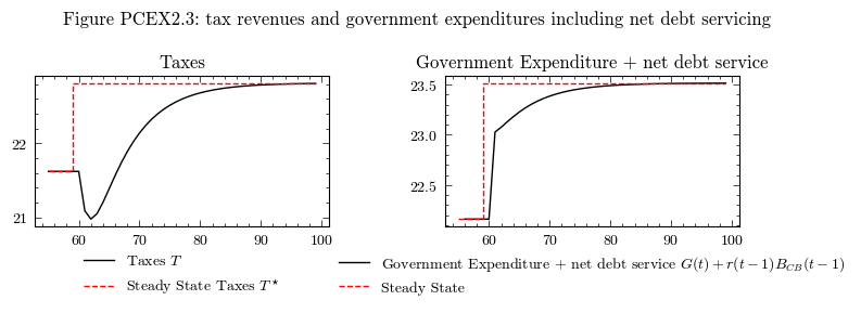
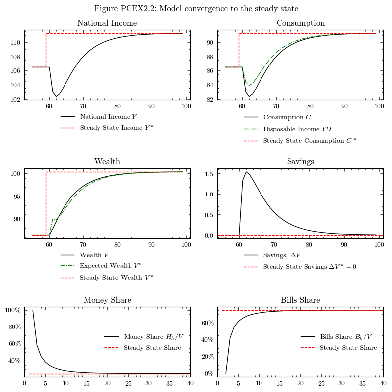
Perturbation 1: An increase of 100 points in the rate of interest on bills (\(r\))#

Following the convergence to the steady state, we can study the effects of an increase in the rate on bills by 100bps (Figures 4.3 and 4.4 in Godley and Lavoie [2006]).

MacroStat is set up to easily handle these scenarios. Much like in prior models, we simply define a new scenario IncreaseInterestRate and set the new rate to be 100 points higher \(r=0.025+0.01\)

model.parameters["scenario_trigger"] = 60
model.scenarios.add_scenario(
    name="IncreaseInterestRate",
    timeseries={"InterestRate":0.025 + 0.01}
)
model.simulate(scenario="IncreaseInterestRate")
output_rate_increase = model.variables.to_pandas()

INFO:root:Starting simulation. Scenario: 1

We then need to compute the new steady state values for the variables

model.compute_theoretical_steady_state(scenario="IncreaseInterestRate")
steadystate_rate_increase = model.variables.to_pandas()

INFO:root:Computing theoretical steady state. Scenario: 1

Now we can see how the model reacts to the shock.

Show code cell source

Hide code cell source

dfo = output_rate_increase.loc[55:]
dfs = steadystate_rate_increase.loc[55:]

fig, axs = plt.subplots(ncols=2, nrows=3, figsize=(8, 8))

# National Income and Consumption
axs[0,0].plot(dfo.index, dfo['NationalIncome'], color='k', label=r'National Income $Y$')
axs[0,0].step(x=dfs.index,y=dfs["NationalIncome"], color='r', linestyle='--', label=r'Steady State Income $Y^\star$')
axs[0,0].legend(loc='upper center', bbox_to_anchor=(0.5, -0.1), frameon=False)
axs[0,0].set_title('National Income')
axs[0,1].plot(dfo.index, dfo['ConsumptionHousehold'], color='k', label=r'Consumption $C$')
axs[0,1].plot(dfo.index, dfo['DisposableIncome'], color='g', linestyle='-.', label=r'Disposable Income $YD$')
axs[0,1].step(x=dfs.index,y=dfs["ConsumptionHousehold"], color='r', linestyle='--', label=r'Steady State Consumption $C^\star$')
axs[0,1].legend(loc='upper center', bbox_to_anchor=(0.5, -0.1), frameon=False)
axs[0,1].set_title('Consumption')

# Wealth and Savings
axs[1,0].plot(dfo.index, dfo['Wealth'], color='k', label=r'Wealth $V$')
axs[1,0].plot(dfo.index, dfo['ExpectedWealth'], color='g', linestyle='-.', label=r'Expected Wealth $V^e$')
axs[1,0].step(x=dfs.index,y=dfs["Wealth"], color='r', linestyle='--', label=r'Steady State Wealth $V^\star$')
axs[1,0].legend(loc='upper center', bbox_to_anchor=(0.5, -0.1), frameon=False)
axs[1,0].set_title('Wealth')
axs[1,1].plot(dfo.index, dfo['Wealth'].diff(), color='k', label=r'Savings, $\Delta V$')
axs[1,1].axhline(y=0, color='r', linestyle='--', label=r'Steady State Savings $\Delta V^\star=0$')
axs[1,1].legend(loc='upper center', bbox_to_anchor=(0.5, -0.1), frameon=False)
axs[1,1].set_title('Savings')

# Money Share and Bills Share
share_bills = steadystate['HouseholdBillStock'] / steadystate['Wealth']
axs[2,0].plot(output.index, output['HouseholdMoneyStock'] / output['Wealth'], color='k', linestyle='-', label='Money Share $H_h/V$')
axs[2,0].step(x=share_bills.index,y=1-share_bills, color='r', linestyle='--', label='Steady State Share')
axs[2,0].legend(loc='center right', frameon=False)
axs[2,0].set_xlim(0,40)
axs[2,0].set_title('Money Share')
axs[2,0].yaxis.set_major_formatter(PercentFormatter(1))

# Right panel - Bills share
axs[2,1].plot(output.index, output['HouseholdBillStock'] / output['Wealth'], color='k', linestyle='-', label='Bills Share $B_h/V$')
axs[2,1].step(x=share_bills.index,y=share_bills, color='r', linestyle='--', label='Steady State Share')
axs[2,1].legend(loc='center right', frameon=False)
axs[2,1].set_xlim(0,40)
axs[2,1].set_title('Bills Share')
axs[2,1].yaxis.set_major_formatter(PercentFormatter(1))


fig.suptitle('Figure PCEX2.2: Model convergence to the steady state')
plt.tight_layout()
plt.show()

../../_images/ebe3fc3c0f929fc00b268300677454dc94a467bf9b8144e58d305483cb7eedd9.png

dfo = output_rate_increase.loc[55:]
dfs = steadystate_rate_increase.loc[55:]

fig, axs = plt.subplots(ncols=2, nrows=1, figsize=(8, 3))

# National Income and Consumption
axs[0].plot(dfo.index, dfo['Taxes'], color='k', label=r'Taxes $T$')
axs[0].step(x=dfs.index,y=dfs["Taxes"], color='r', linestyle='--', label=r'Steady State Taxes $T^\star$')
axs[0].legend(loc='upper center', bbox_to_anchor=(0.5, -0.1), frameon=False)
axs[0].set_title('Taxes')
# Government Expenditure + net debt service
gov = dfo['ConsumptionGovernment'] + (dfo["InterestRate"] * dfo["GovernmentBillStock"]).shift(1)
gov_ss = dfs['ConsumptionGovernment'] + (dfs["InterestRate"] * dfs["GovernmentBillStock"])
axs[1].plot(dfo.index, gov, color='k', label=r'Government Expenditure + net debt service $G(t) + r(t-1)B_{CB}(t-1)$')
axs[1].step(x=dfs.index,y=gov_ss, color='r', linestyle='--', label=r'Steady State')
axs[1].legend(loc='upper center', bbox_to_anchor=(0.5, -0.1), frameon=False)
axs[1].set_title('Government Expenditure + net debt service')

fig.suptitle('Figure PCEX2.3: tax revenues and government expenditures including net debt servicing')
plt.tight_layout()
plt.show()

../../_images/9e77436b66552da92d81e5e916091d3e6e7b6531d2e638b1c7ba29814792cb96.png