Mark-0 COVID Heterogeneous-Agent ABM

Mark-0 is a closed-economy ABM with \(N\) firms, one representative household, one commercial bank, and one central bank. The COVID extension [] adds the parameter set used to study V-, U-, L-, and W-shaped recovery regimes. Each macro period executes an ordered 24-phase loop: price/wage adjustment, hiring/firing, production, household consumption, interest-rate setting, bankruptcy, and firm revival.

Stochastic phases are reparameterised through three independent frozen \(U(0, 1)\) noise buffers of shape (timesteps, N_firms) pre-drawn in initialize(). Boundary conditions on the two gradient-critical paths (stay_alive indicator and the positive-\(Y\) guard) use Behavior.diffwhere; all other branches use plain torch.where, matching the abmstat reference pattern.

Module Contents

Mark0COVID is divided into Variables, Parameters (fixed constants), Scenarios, and the Behavior (model initialization and steps). See the sibling pages linked from the model index for the per-component tables.

Implementation in MacroStat

The forward pass is differentiable end-to-end. The 24-phase loop is decomposed into named methods on BehaviorMark0COVID so that each phase carries its own docstring and Equations section. ParametersMark0COVID.get_default_hyperparameters sets dtype = torch.float64 to match the abmstat reference precision.

Model Dynamics

Preparatory Steps

%load_ext autoreload
%autoreload 2

import importlib
import logging
import sys

from matplotlib import pyplot as plt

from macrostat.models.Mark0COVID import Mark0COVID, ParametersMark0COVID

plt.style.use("../../macrostat.mplstyle")
importlib.reload(logging)
logging.basicConfig(stream=sys.stdout, level=logging.INFO)

Four Gualdi phases

show that the Mark-0 long-run regime is determined by the location of \((R, \Theta)\) in the parameter plane, where \(R = \eta_+/\eta_-\) is the hiring/firing asymmetry and \(\Theta\) is the bankruptcy default threshold. Four phases occupy distinct regions:

• FU (Full Unemployment): \(R < R_c\), the economy collapses to near-zero employment regardless of \(\Theta\).

• RU (Residual Unemployment): \(R > R_c\), low \(\Theta\); firms default quickly so a non-trivial unemployment rate persists.

• EC (Endogenous Crises): \(R > R_c\), intermediate \(\Theta\); bankruptcy cascades trigger large oscillations between near-FE and near-FU regimes.

• FE (Full Employment): \(R > R_c\), large \(\Theta\); defaults are rare and the economy sits near full employment.

Each phase is realised as a distinct ParametersMark0COVID instance varying HiringFiringRate (\(R\)) and DefaultThreshold (\(\Theta\)) only; all other parameters take their default values.

phases = {
    "FU (R=0.5, Theta=3)": (0.5, 3.0),
    "RU (R=2, Theta=0.5)": (2.0, 0.5),
    "EC (R=2, Theta=1.2)": (2.0, 1.2),
    "FE (R=2, Theta=5)": (2.0, 5.0),
}

paths = {}
for label, (R, Theta) in phases.items():
    params = ParametersMark0COVID(
        hyperparameters={"timesteps": 1000, "N_firms": 10000, "seed": 0},
    )
    params["HiringFiringRate"] = R
    params["DefaultThreshold"] = Theta
    model = Mark0COVID(parameters=params)
    model.simulate()
    paths[label] = model.variables.to_pandas()

Unemployment trajectory

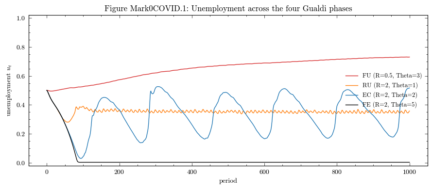
The aggregate unemployment series isolates the four phases at a glance. FU collapses to \(u \to 1\); RU settles at a positive residual; EC oscillates between near-FE and near-FU bands; FE converges close to full employment.

fig, ax = plt.subplots(figsize=(9, 4))
colors = ["tab:red", "tab:orange", "tab:blue", "k"]

for color, (label, df) in zip(colors, paths.items()):
    ax.plot(df.index, df["Unemployment"], color=color, linewidth=1.0, label=label)

ax.set_title("Figure Mark0COVID.1: Unemployment across the four Gualdi phases")
ax.set_xlabel("period")
ax.set_ylabel(r"unemployment $u_t$")
ax.set_ylim(-0.02, 1.02)
ax.legend(loc="center right", frameon=False, fontsize=9)
plt.tight_layout()
plt.show()

Notes

• The shape of every het-agent state tensor in model.variables.timeseries is (T + 1, N_firms); aggregates are stored as (T + 1, 1). to_pandas() returns a multi-column DataFrame indexed by time.