NK3E

The New Keynesian 3-Equation (NK3E) model is a compact framework for analyzing the joint dynamics of output, inflation, and the real interest rate. It is based on and follows the implementation at macrosimulation.org.

The model captures three core mechanisms:

1. Demand (IS curve): output depends negatively on the lagged real interest rate.

2. Inflation (Phillips curve): inflation accelerates when output exceeds potential.

3. Monetary policy: the central bank sets the real rate to steer inflation toward its target.

Module Contents

As with all MacroStat models, NK3E is divided into Variables, Parameters (fixed constants), Scenarios, and the Behavior (model initialization and steps). The module-level documentation can be seen in:

• Variables
• Parameters
  • Hyperparameters
  • Parameters
• Equations
  • Step Equations
• Scenarios

The remainder of this page gives an introduction to the model, notes on how it is implemented in MacroStat and then shows some of the model dynamics.

Model Overview

Behavioral Equations

The model consists of three behavioral equations and two derived quantities. All variables are in deviation from some normalisation; output \(y\) is in levels, \(\pi\) is the inflation rate, and \(r\) is the real interest rate.

1. IS curve — output as a function of autonomous demand and the lagged real rate

\[ y_t = A - a_1 \, r_{t-1} \]

2. Phillips curve — inflation responds to the output gap

\[ \pi_t = \pi_{t-1} + a_2 \, (y_t - y_e) \]

3. Stabilizing real rate — the rate consistent with output at potential

\[ r_s = \frac{A - y_e}{a_1} \]

4. Central bank response slope — derived from the loss-minimizing policy

\[ a_3 = \frac{1}{a_1 \left( \dfrac{1}{a_2 b} + a_2 \right)} \]

5. Monetary policy rule — the real rate reacts to inflation deviations

\[ r_t = r_s + a_3 \, (\pi_t - \pi^T) \]

At steady state, \(y = y_e\), \(\pi = \pi^T\), and \(r = r_s\).

Implementation in MacroStat

Transposing these equations to the MacroStat framework, we consider that there are:

1. Six parameters (fixed constants): \(a_1\), \(a_2\), \(b\), \(A\), \(\pi^T\), \(y_e\) (see Parameters)

2. Six scenario keys divided into two families (see Scenarios):

   • Parameter-step shocks (A_add, pi_T_add, y_e_add): additive offsets applied to structural parameters from scenario_trigger onward.

   • State-variable shocks (InflationShock, RateShock, OutputShock): additive perturbations applied directly to \(\pi\), \(r\), \(y\) inside BehaviorNK3E.step. These default to zero; Scenario.4 registers a one-period impulse on \(\pi\). OutputShock and RateShock follow the same pattern and are available but not exercised here.

3. Five tracked variables: \(y\), \(\pi\), \(r\), \(r_s\), \(a_3\) (see Variables)

The derived quantities \(r_s\) and \(a_3\) are recomputed every period from the (possibly shocked) parameters, so they respond immediately to parameter-step shocks. State-variable shocks bypass the parameter layer and perturb the system directly within a single period.

Model Dynamics

Preparatory Steps

%load_ext autoreload
%autoreload 2

import importlib
import logging
import sys

from matplotlib import pyplot as plt

from macrostat.models.NK3E import NK3E, ParametersNK3E, ScenariosNK3E

plt.style.use("../../macrostat.mplstyle")
importlib.reload(logging)
logging.basicConfig(stream=sys.stdout, level=logging.INFO)

Running the Simulation

First, we run the model without any shocks to see the convergence to the steady state. We set a scenario trigger at \(t = 25\) so that later perturbation experiments show a clear pre-shock baseline.

params = ParametersNK3E(hyperparameters={"timesteps": 70, "scenario_trigger": 25})
model = NK3E(parameters=params)
model.simulate()
output = model.variables.to_pandas()

We can check that the variables are healthy (redundant equation holds, stocks are positive):

model.variables.check_health()

Check health not implemented for this model

True

An overview of the first 10 steps of the model:

output.head(10).T

	time	0	1	2	3	4	5	6	7	8	9
y	Macroeconomy	5.000000	5.000000	5.000000	5.000000	5.000000	5.000000	5.000000	5.000000	5.000000	5.000000
a3	Macroeconomy	1.565995	1.565995	1.565995	1.565995	1.565995	1.565995	1.565995	1.565995	1.565995	1.565995
pi	Macroeconomy	2.000000	2.000000	2.000000	2.000000	2.000000	2.000000	2.000000	2.000000	2.000000	2.000000
r	Macroeconomy	16.666666	16.666666	16.666666	16.666666	16.666666	16.666666	16.666666	16.666666	16.666666	16.666666
r_s	Macroeconomy	16.666666	16.666666	16.666666	16.666666	16.666666	16.666666	16.666666	16.666666	16.666666	16.666666

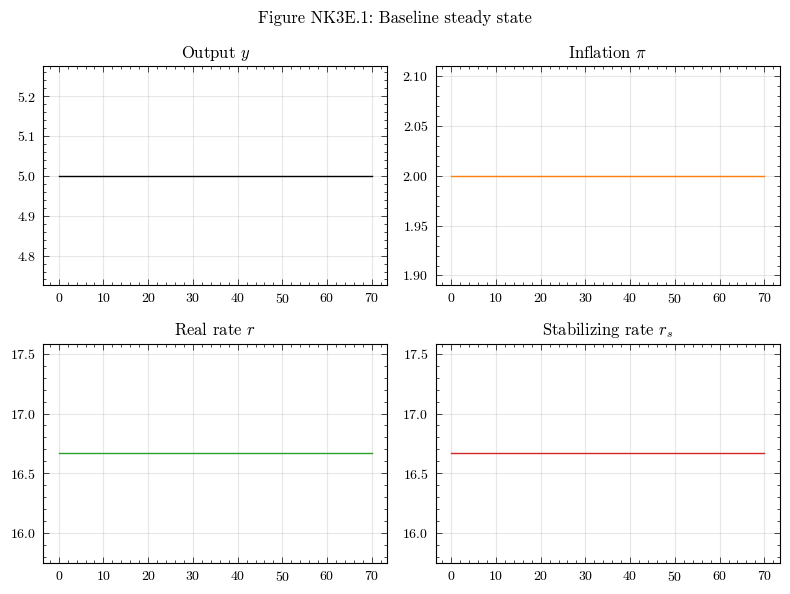
Convergence to the Steady State

Without shocks, the NK3E model sits at its analytical steady state from the first period: \(y = y_e = 5\), \(\pi = \pi^T = 2\), and \(r = r_s = (A - y_e) / a_1 \approx 16.67\). The flat lines below confirm that the numerical simulation reproduces this exactly.

fig, axs = plt.subplots(ncols=2, nrows=2, figsize=(8, 6))

axs[0, 0].plot(output.index, output["y"], color="k")
axs[0, 0].set_title(r"Output $y$")

axs[0, 1].plot(output.index, output["pi"], color="tab:orange")
axs[0, 1].set_title(r"Inflation $\pi$")

axs[1, 0].plot(output.index, output["r"], color="tab:green")
axs[1, 0].set_title(r"Real rate $r$")

axs[1, 1].plot(output.index, output["r_s"], color="tab:red")
axs[1, 1].set_title(r"Stabilizing rate $r_s$")

for ax in axs.ravel():
    ax.grid(True, alpha=0.3)

fig.suptitle("Figure NK3E.1: Baseline steady state")
plt.tight_layout()
plt.show()

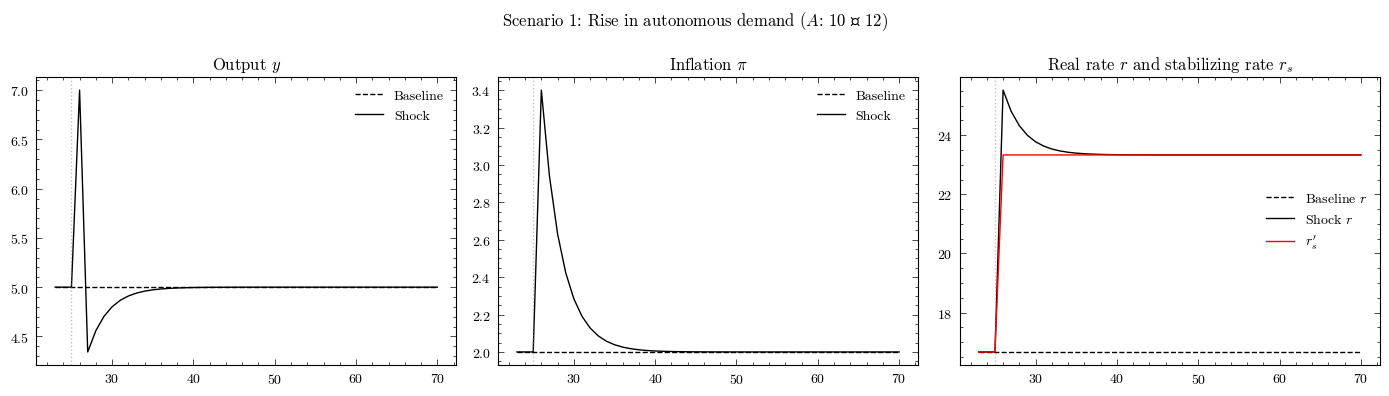
Perturbation 1: Rise in autonomous demand (\(A\))

A permanent increase in autonomous demand (\(A\): 10 \(\to\) 12) shifts the IS curve to the right. Output jumps above potential, the Phillips curve pushes inflation up, and the central bank raises the real rate above the new (higher) stabilizing rate to bring inflation back to target. In the long run, the economy converges to a new steady state with the same \(y_e\) and \(\pi^T\) but a higher stabilizing real rate \(r_s^\prime = (A^\prime - y_e) / a_1\).

scenarios = ScenariosNK3E(parameters=params)
sc1 = scenarios.get_scenario_index("Scenario.1: Rise in A")
model_sc1 = NK3E(parameters=params, scenarios=scenarios)
model_sc1.simulate(scenario=sc1)
output_sc1 = model_sc1.variables.to_pandas()

trigger = params["scenario_trigger"]
t_slice = slice(trigger - 2, None)

fig, axs = plt.subplots(1, 3, figsize=(14, 4))

axs[0].plot(
    output.loc[t_slice].index, output.loc[t_slice, "y"], "k--", label="Baseline"
)
axs[0].plot(
    output_sc1.loc[t_slice].index, output_sc1.loc[t_slice, "y"], "k-", label="Shock"
)
axs[0].axvline(x=trigger, color="grey", linestyle=":", alpha=0.5)
axs[0].set_title(r"Output $y$")
axs[0].legend(frameon=False)

axs[1].plot(
    output.loc[t_slice].index, output.loc[t_slice, "pi"], "k--", label="Baseline"
)
axs[1].plot(
    output_sc1.loc[t_slice].index, output_sc1.loc[t_slice, "pi"], "k-", label="Shock"
)
axs[1].axvline(x=trigger, color="grey", linestyle=":", alpha=0.5)
axs[1].set_title(r"Inflation $\pi$")
axs[1].legend(frameon=False)

axs[2].plot(
    output.loc[t_slice].index, output.loc[t_slice, "r"], "k--", label="Baseline $r$"
)
axs[2].plot(
    output_sc1.loc[t_slice].index, output_sc1.loc[t_slice, "r"], "k-", label="Shock $r$"
)
axs[2].plot(
    output_sc1.loc[t_slice].index,
    output_sc1.loc[t_slice, "r_s"],
    "r-",
    label=r"$r_s^\prime$",
)
axs[2].axvline(x=trigger, color="grey", linestyle=":", alpha=0.5)
axs[2].set_title(r"Real rate $r$ and stabilizing rate $r_s$")
axs[2].legend(frameon=False)

fig.suptitle("Scenario 1: Rise in autonomous demand ($A$: 10 → 12)")
plt.tight_layout()
plt.show()

Font 'default' does not have a glyph for '\u2192' [U+2192], substituting with a dummy symbol.

Font 'default' does not have a glyph for '\u2192' [U+2192], substituting with a dummy symbol.

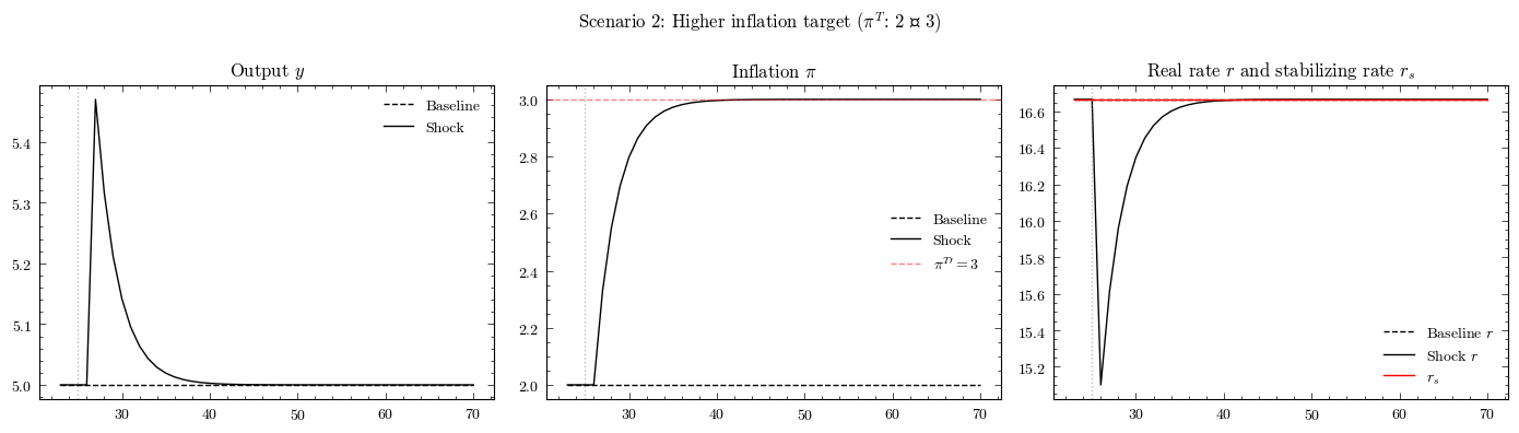
Perturbation 2: Higher inflation target (\(\pi^T\))

A permanent increase in the inflation target (\(\pi^T\): 2 \(\to\) 3) does not change the stabilizing real rate \(r_s\) (which depends on \(A\), \(y_e\), \(a_1\) only). However, the monetary policy rule now targets a higher inflation rate. Since the current inflation rate starts below the new target, the central bank initially cuts the real rate below \(r_s\). This stimulates output above potential, which drives inflation upward. The economy converges to the new steady state with \(\pi = \pi^{T\prime} = 3\), \(y = y_e\), and \(r = r_s\) (unchanged).

sc2 = scenarios.get_scenario_index("Scenario.2: Higher pi_T")
model_sc2 = NK3E(parameters=params, scenarios=scenarios)
model_sc2.simulate(scenario=sc2)
output_sc2 = model_sc2.variables.to_pandas()

fig, axs = plt.subplots(1, 3, figsize=(14, 4))

axs[0].plot(
    output.loc[t_slice].index, output.loc[t_slice, "y"], "k--", label="Baseline"
)
axs[0].plot(
    output_sc2.loc[t_slice].index, output_sc2.loc[t_slice, "y"], "k-", label="Shock"
)
axs[0].axvline(x=trigger, color="grey", linestyle=":", alpha=0.5)
axs[0].set_title(r"Output $y$")
axs[0].legend(frameon=False)

axs[1].plot(
    output.loc[t_slice].index, output.loc[t_slice, "pi"], "k--", label="Baseline"
)
axs[1].plot(
    output_sc2.loc[t_slice].index, output_sc2.loc[t_slice, "pi"], "k-", label="Shock"
)
axs[1].axhline(y=3.0, color="r", linestyle="--", alpha=0.5, label=r"$\pi^{T\prime}=3$")
axs[1].axvline(x=trigger, color="grey", linestyle=":", alpha=0.5)
axs[1].set_title(r"Inflation $\pi$")
axs[1].legend(frameon=False)

axs[2].plot(
    output.loc[t_slice].index, output.loc[t_slice, "r"], "k--", label="Baseline $r$"
)
axs[2].plot(
    output_sc2.loc[t_slice].index, output_sc2.loc[t_slice, "r"], "k-", label="Shock $r$"
)
axs[2].plot(
    output_sc2.loc[t_slice].index, output_sc2.loc[t_slice, "r_s"], "r-", label=r"$r_s$"
)
axs[2].axvline(x=trigger, color="grey", linestyle=":", alpha=0.5)
axs[2].set_title(r"Real rate $r$ and stabilizing rate $r_s$")
axs[2].legend(frameon=False)

fig.suptitle(r"Scenario 2: Higher inflation target ($\pi^T$: 2 → 3)")
plt.tight_layout()
plt.show()

Font 'default' does not have a glyph for '\u2192' [U+2192], substituting with a dummy symbol.

Font 'default' does not have a glyph for '\u2192' [U+2192], substituting with a dummy symbol.

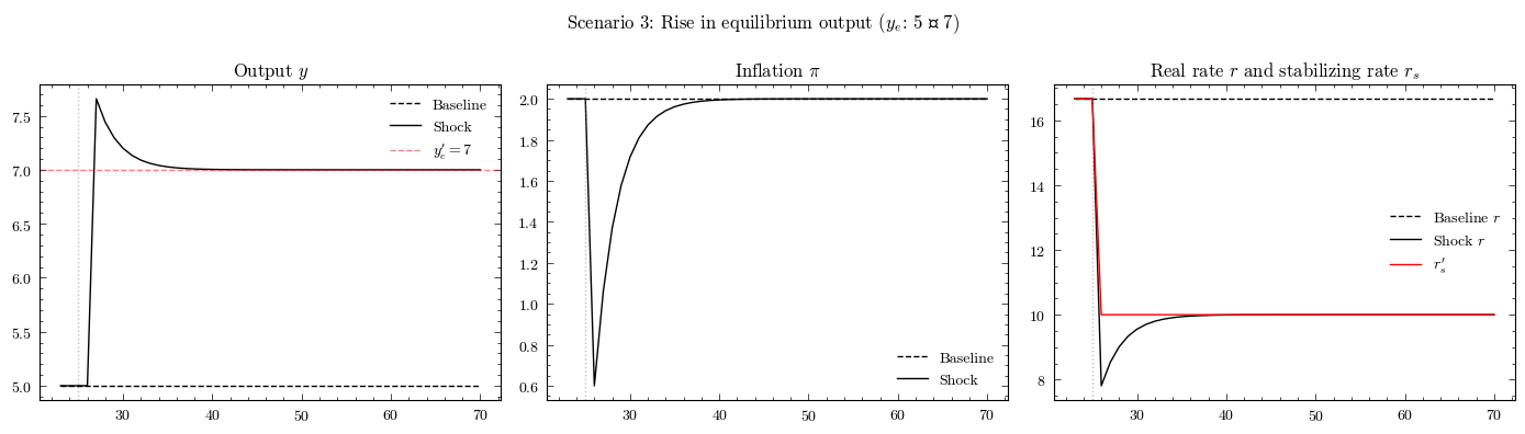
Perturbation 3: Rise in equilibrium output (\(y_e\))

A permanent increase in equilibrium output (\(y_e\): 5 \(\to\) 7) represents a positive supply-side shock. The stabilizing real rate falls because the same autonomous demand \(A\) now needs a lower rate to clear the goods market at the higher potential. Output initially undershoots the new potential (since \(r\) was calibrated to the old \(y_e\)), which pushes inflation below target. The central bank lowers the rate, and the economy converges to the new steady state with \(y = y_e^\prime = 7\), \(\pi = \pi^T\), and a lower \(r_s^\prime = (A - y_e^\prime) / a_1\).

sc3 = scenarios.get_scenario_index("Scenario.3: Rise in y_e")
model_sc3 = NK3E(parameters=params, scenarios=scenarios)
model_sc3.simulate(scenario=sc3)
output_sc3 = model_sc3.variables.to_pandas()

fig, axs = plt.subplots(1, 3, figsize=(14, 4))

axs[0].plot(
    output.loc[t_slice].index, output.loc[t_slice, "y"], "k--", label="Baseline"
)
axs[0].plot(
    output_sc3.loc[t_slice].index, output_sc3.loc[t_slice, "y"], "k-", label="Shock"
)
axs[0].axhline(y=7.0, color="r", linestyle="--", alpha=0.5, label=r"$y_e^\prime=7$")
axs[0].axvline(x=trigger, color="grey", linestyle=":", alpha=0.5)
axs[0].set_title(r"Output $y$")
axs[0].legend(frameon=False)

axs[1].plot(
    output.loc[t_slice].index, output.loc[t_slice, "pi"], "k--", label="Baseline"
)
axs[1].plot(
    output_sc3.loc[t_slice].index, output_sc3.loc[t_slice, "pi"], "k-", label="Shock"
)
axs[1].axvline(x=trigger, color="grey", linestyle=":", alpha=0.5)
axs[1].set_title(r"Inflation $\pi$")
axs[1].legend(frameon=False)

axs[2].plot(
    output.loc[t_slice].index, output.loc[t_slice, "r"], "k--", label="Baseline $r$"
)
axs[2].plot(
    output_sc3.loc[t_slice].index, output_sc3.loc[t_slice, "r"], "k-", label="Shock $r$"
)
axs[2].plot(
    output_sc3.loc[t_slice].index,
    output_sc3.loc[t_slice, "r_s"],
    "r-",
    label=r"$r_s^\prime$",
)
axs[2].axvline(x=trigger, color="grey", linestyle=":", alpha=0.5)
axs[2].set_title(r"Real rate $r$ and stabilizing rate $r_s$")
axs[2].legend(frameon=False)

fig.suptitle(r"Scenario 3: Rise in equilibrium output ($y_e$: 5 → 7)")
plt.tight_layout()
plt.show()

Font 'default' does not have a glyph for '\u2192' [U+2192], substituting with a dummy symbol.

Font 'default' does not have a glyph for '\u2192' [U+2192], substituting with a dummy symbol.

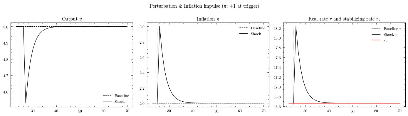
Perturbation 4: Inflation impulse

The first three perturbations change a structural parameter permanently from scenario_trigger onward. This perturbation differs in kind. It injects a one-period additive shock of \(+1\) directly into \(\pi_t\) at the trigger, leaving all parameters unchanged. After that single period the shock value returns to zero and the model evolves freely.

Economically, this captures an exogenous inflation surprise — a cost-push impulse or an expectation shock — not driven by any change in demand, potential output, or the inflation target. The structural parameters \(A\), \(y_e\), and \(\pi^T\) are identical to the baseline throughout, so \(r_s\) and \(a_3\) are unaffected.

The expected dynamics follow from the three equations. In the shock period \(\pi_t\) rises by \(+1\). The monetary policy rule raises \(r_t\) above \(r_s\). In the next period the higher \(r\) suppresses output via the IS curve, the negative output gap pulls \(\pi\) back toward target, and the central bank relaxes the rate. The economy converges monotonically to the original steady state with no permanent shift in any variable.

sc4 = scenarios.get_scenario_index("Scenario.4: Inflation impulse")
model_sc4 = NK3E(parameters=params, scenarios=scenarios)
model_sc4.simulate(scenario=sc4)
output_sc4 = model_sc4.variables.to_pandas()

fig, axs = plt.subplots(1, 3, figsize=(14, 4))

axs[0].plot(
    output.loc[t_slice].index, output.loc[t_slice, "y"], "k--", label="Baseline"
)
axs[0].plot(
    output_sc4.loc[t_slice].index, output_sc4.loc[t_slice, "y"], "k-", label="Shock"
)
axs[0].axvline(x=trigger, color="grey", linestyle=":", alpha=0.5)
axs[0].set_title(r"Output $y$")
axs[0].legend(frameon=False)

axs[1].plot(
    output.loc[t_slice].index, output.loc[t_slice, "pi"], "k--", label="Baseline"
)
axs[1].plot(
    output_sc4.loc[t_slice].index, output_sc4.loc[t_slice, "pi"], "k-", label="Shock"
)
axs[1].axvline(x=trigger, color="grey", linestyle=":", alpha=0.5)
axs[1].set_title(r"Inflation $\pi$")
axs[1].legend(frameon=False)

axs[2].plot(
    output.loc[t_slice].index, output.loc[t_slice, "r"], "k--", label="Baseline $r$"
)
axs[2].plot(
    output_sc4.loc[t_slice].index, output_sc4.loc[t_slice, "r"], "k-", label="Shock $r$"
)
axs[2].plot(
    output_sc4.loc[t_slice].index, output_sc4.loc[t_slice, "r_s"], "r-", label=r"$r_s$"
)
axs[2].axvline(x=trigger, color="grey", linestyle=":", alpha=0.5)
axs[2].set_title(r"Real rate $r$ and stabilizing rate $r_s$")
axs[2].legend(frameon=False)

fig.suptitle(r"Perturbation 4: Inflation impulse ($\pi$: $+1$ at trigger)")
plt.tight_layout()
plt.show()