Model INSOUT

Model INSOUT is introduced in Chapter 10 (2nd ed.) / Chapter 7 (1st ed.) of Godley and Lavoie [2006] “Monetary Economics: An Integrated Approach to Credit, Money, Income, Production and Wealth”. It extends the LP family of models by introducing a full production sector with inventories, endogenous bank interest rates, wage-price dynamics, and a five-sector economy (Household, Firm, Government, Central Bank, Bank).

Module Contents

As with all MacroStat models, INSOUT is divided into Variables, Parameters (fixed constants), Scenarios, and the Behavior (model initialization and steps). The module-level documentation can be seen in:

• Variables
• Parameters
  • Hyperparameters
  • Parameters
• Equations
  • Step Equations
• Scenarios
  • Baseline
  • Scenario 1: Higher Target Inventory Ratio (INSOUT1)
  • Scenario 2: Higher Government Spending (INSOUT2)
  • Scenario 3: Higher Reserve Requirements (INSOUT3)
  • Scenario 4: Wider Bank Liquidity Corridor (INSOUT4)
  • Scenario 5: Lower Consumption Propensity (INSOUT5)
  • Scenario 6: Exogenous Increase in Inflation via Wage Target (INSOUT6)
  • Scenario 7: Combined Wage Push and Interest Rate Increase (INSOUT7)

The remainder of this page gives an introduction to the model, notes on how it is implemented in MacroStat and then shows some of the model dynamics across different scenarios.

Model Overview

Behavioral Equations

Model INSOUT introduces production with inventories, endogenous bank rates, and wage-price dynamics into the SFC framework. The key features are:

• Firms produce output, hold inventories financed by bank loans, and set prices as a markup over normal historic unit cost (including an indirect production tax)

• Banks set deposit and loan rates endogenously based on liquidity and profitability corridors

• Households allocate wealth across four non-cash assets (M1, M2, bills, bonds) using Tobin portfolio choice

• Wage-price dynamics with a Phillips-curve-style target real wage and partial adjustment

Firm Expectations and Pricing

1. Expected sales (adaptive expectations) $\( s^e(t) = \beta \cdot s(t-1) + (1 - \beta) \cdot s^e(t-1) \)$

2. Target inventory-sales ratio $\( \sigma^T(t) = \sigma_0 - \sigma_1 \cdot r_l(t) \)$

3. Target inventories $\( inv^T(t) = \sigma^T(t) \cdot s^e(t) \)$

4. Expected inventories (partial adjustment) $\( inv^e(t) = inv(t-1) - \gamma \cdot (inv(t-1) - inv^T(t)) \)$

5. Normal historic unit cost $\( NHUC(t) = (1 - \sigma^T) \cdot UC(t-1) + \sigma^T \cdot (1 + r_l(t-1)) \cdot UC(t-1) \)$

6. Price level (including indirect tax) $\( p(t) = (1 + \tau) \cdot (1 + \phi) \cdot NHUC(t) \)$

7. Inflation rate $\( \pi(t) = \frac{p(t) - p(t-1)}{p(t-1)} \)$

Firm Realized Outcomes

8. Real sales $\( s(t) = c(t) + g(t) \)$

9. Nominal sales $\( S(t) = s(t) \cdot p(t) \)$

10. Indirect production tax $\( TX(t) = \frac{\tau}{1 + \tau} \cdot S(t) \)$

11. Real inventories $\( inv(t) = inv(t-1) + y(t) - s(t) \)$

12. Nominal inventories (valued at unit cost) $\( INV(t) = inv(t) \cdot UC(t) \)$

13. Loan demand $\( L^d(t) = INV(t) \)$

14. Firm profits $\( FP(t) = S(t) - TX(t) - WB(t) + (INV(t) - INV(t-1)) - r_l(t-1) \cdot L_s(t-1) \)$

15. Nominal output (sales at price + inventory change at cost) $\( Y(t) = p(t) \cdot s(t) + UC(t) \cdot (inv(t) - inv(t-1)) \)$

Household Behavioral

16. Real consumption $\( c(t) = \alpha_0 + \alpha_1 \cdot yd_r^e(t) + \alpha_2 \cdot v(t-1) \)$

17. Expected real disposable income $\( yd_r^e(t) = \varepsilon \cdot yd_r(t-1) + (1 - \varepsilon) \cdot yd_r^e(t-1) \)$

18. Nominal expected disposable income (with inflation adjustment) $\( YD^e(t) = yd_r^e(t) \cdot p(t) + \pi(t) \cdot \frac{V(t-1)}{p(t)} \)$

19. Expected nominal wealth $\( V^e(t) = V(t-1) + YD^e(t) - C(t) \)$

20. Cash demand $\( Hh^d(t) = \lambda_c \cdot C(t) \)$

21. Expected non-cash wealth $\( V^e_{nc}(t) = V^e(t) - Hh^d(t) \)$

Household Realized

22. Regular disposable income (no explicit tax; indirect tax netted in firm profits) $\( YD_r(t) = WB(t) + FD(t) + r_m(t-1) \cdot M2_h(t-1) + r_b(t-1) \cdot B_h(t-1) + BL_h(t-1) \)$

23. Real regular disposable income (with inflation erosion) $\( yd_r(t) = \frac{YD_r(t)}{p(t)} - \pi(t) \cdot \frac{V(t-1)}{p(t)} \)$

24. Capital gains $\( CG(t) = (p_{bl}(t) - p_{bl}(t-1)) \cdot BL_h(t-1) \)$

25. Haig-Simons disposable income $\( YD_{hs}(t) = YD_r(t) + CG(t) \)$

26. Nominal wealth $\( V(t) = V(t-1) + YD_{hs}(t) - C(t) \)$

Portfolio Allocation

27. M2 demand, Bills demand, Bonds demand (Tobin portfolio allocation) $\( M2^d(t) = V^e_{nc} \cdot (\lambda_{20} + \lambda_{22} \cdot r_m + \lambda_{23} \cdot r_b + \lambda_{24} \cdot ERr_{bl}) + \lambda_{25} \cdot YD^e \)$

\[ B^d(t) = V^e_{nc} \cdot (\lambda_{30} + \lambda_{32} \cdot r_m + \lambda_{33} \cdot r_b + \lambda_{34} \cdot ERr_{bl}) + \lambda_{35} \cdot YD^e \]

\[ BL^d(t) = \frac{V^e_{nc} \cdot (\lambda_{40} + \lambda_{42} \cdot r_m + \lambda_{43} \cdot r_b + \lambda_{44} \cdot ERr_{bl}) + \lambda_{45} \cdot YD^e}{p_{bl}(t)} \]

28. M1 demand (buffer-stock residual of actual non-cash wealth) $\( M1^d(t) = V_{nc}(t) - M2^d(t) - B^d(t) - p_{bl}(t) \cdot BL^d(t) \)$

where \(V_{nc} = V - Hh^d\) is actual (not expected) non-cash wealth.

29. M1/M2 switching regime: \(z_1 = 1\) if \(M1^d > 0\), else \(z_2 = 1\) and M2 absorbs the residual.

Government

30. Government spending $\( G(t) = g(t) \cdot p(t) \)$

31. Public sector borrowing requirement $\( PSBR(t) = G(t) + r_b(t-1) \cdot B_s(t-1) + BL_s(t-1) - TX(t) - FCB(t) \)$

32. Bill supply (residual financing) $\( B_s(t) = B_s(t-1) + PSBR(t) - (BL_s(t) - BL_s(t-1)) \cdot p_{bl}(t) \)$

Central Bank

33. Central bank profits $\( FCB(t) = r_b(t-1) \cdot B_{cb}(t-1) + r_a(t-1) \cdot A_s(t-1) \)$

34. Advances supply $\( A_s(t) = A^d(t) \)$

35. Central bank bill holdings (residual) $\( B_{cb}(t) = B_s(t) - B_h(t) - B_b(t) \)$

Banks

36. Bank profits $\( FBP(t) = r_l(t-1) \cdot L_s(t-1) + r_b(t-1) \cdot B_b(t-1) - r_m(t-1) \cdot M2_s(t-1) - r_a(t-1) \cdot A_s(t-1) \)$

37. Required reserves $\( RR(t) = \rho_1 \cdot M1_s(t) + \rho_2 \cdot M2_s(t) \)$

38. Tentative bank bill holdings $\( B_b^T(t) = M1_s + M2_s - L_s - Hb_s \)$

39. Advances demand (if \(BLR^T < bot\)) $\( A^d(t) = \max(bot \cdot (M1_s + M2_s) - B_b^T, 0) \cdot z_3 \)$

Endogenous Interest Rates

40. Deposit rate $\( r_m(t) = r_m(t-1) + \zeta_m \cdot (z_4 - z_5) + \zeta_b \cdot (r_b(t) - r_b(t-1)) \)$

41. Loan rate $\( r_l(t) = r_l(t-1) + \zeta_l \cdot (z_6 - z_7) + (r_b(t) - r_b(t-1)) \)$

where \(z_4, z_5\) are liquidity corridor switches (using lagged \(BLR^T\)) and \(z_6, z_7\) are profit corridor switches (using current-period \(BPM\)).

Wage-Price Dynamics

42. Target real wage $\( \omega^T(t) = \exp(\Omega_0 + \Omega_1 \log(pr) + \Omega_2 \log(N(t)/N_{fe})) \)$

43. Nominal wage (partial adjustment to lagged target) $\( W(t) = W(t-1) \cdot (1 + \Omega_3 \cdot (\omega^T(t-1) - W(t-1)/p(t-1))) \)$

Transaction Flow Matrix

Accounting Transaction Matrix for Model INSOUT

	Household	Firm	Government	CentralBank	Bank	Total
	Current	Current	Current	Current	Current
Wage Bill	\(+WB(t)\)	\(-WB(t)\)				\(0\)
Nominal Sales	\(-S(t)\)	\(+S(t)\)				\(0\)
Nominal Consumption	\(-C(t)\)	\(+C(t)\)				\(0\)
Government Spending		\(+G(t)\)	\(-G(t)\)			\(0\)
Taxes		\(-TX(t)\)	\(+TX(t)\)			\(0\)
Total Dividends	\(+FD(t)\)	\(-FD(t)\)				\(0\)
Central Bank Profits			\(+FCB(t)\)	\(-FCB(t)\)		\(0\)
Change in Real Inventories		\(+\Delta inv(t)\)				\(0\)
Change in Nominal Inventories		\(+\Delta INV(t)\)				\(0\)
Change in Cash	\(+\Delta Hh(t)\)					\(0\)
Change in M1	\(+\Delta M1_h(t)\)					\(0\)
Change in M2	\(+\Delta M2_h(t)\)					\(0\)
Change in Bills	\(+\Delta B_h(t)\)			\(+\Delta B_{cb}(t)\)	\(+\Delta B_b(t)\)	\(0\)
Change in Bonds	\(+\Delta BL_h(t)\)					\(0\)
Change in Bonds Supply			\(-\Delta BL_s(t)\)			\(0\)
Change in Bills Supply			\(-\Delta B_s(t)\)			\(0\)
Change in Loans Supply					\(+\Delta L_s(t)\)	\(0\)
Change in M1 Supply					\(-\Delta M1_s(t)\)	\(0\)
Change in M2 Supply					\(-\Delta M2_s(t)\)	\(0\)
Change in Cashs Supply					\(+\Delta Hb_s(t)\)	\(0\)
Change in Advances Supply				\(+\Delta A_s(t)\)		\(0\)
Change in High Powered Money				\(-\Delta H_s(t)\)		\(0\)
Total	\(0\)	\(0\)	\(0\)	\(0\)	\(0\)	\(0\)

Balance Sheet Matrix

Balance Sheet for Model INSOUT

	Household	Firm	Government	CentralBank	Bank	Total
	Current	Current	Current	Current	Current
Real Inventories		\(+inv(t)\)				0
Nominal Inventories		\(+INV(t)\)				0
Nominal Wealth	\(-V(t)\)					0
Cash	\(+Hh(t)\)					0
M1	\(+M1_h(t)\)					0
M2	\(+M2_h(t)\)					0
Bills	\(+B_h(t)\)			\(+B_{cb}(t)\)	\(+B_b(t)\)	0
Bonds	\(+BL_h(t)\)					0
Bonds Supply			\(-BL_s(t)\)			0
Bills Supply			\(-B_s(t)\)			0
Loans Supply					\(+L_s(t)\)	0
M1 Supply					\(-M1_s(t)\)	0
M2 Supply					\(-M2_s(t)\)	0
Cashs Supply					\(+Hb_s(t)\)	0
Advances Supply				\(+A_s(t)\)		0
High Powered Money				\(-H_s(t)\)		0

Implementation in MacroStat

Transposing these equations to the MacroStat framework, we consider that there are:

1. Twenty-eight parameters (fixed constants): consumption propensities (\(\alpha_0\), \(\alpha_1\), \(\alpha_2\)), expectation weights (\(\beta\), \(\gamma\), \(\varepsilon\)), portfolio cash ratio (\(\lambda_c\)), markup (\(\phi\)), tax rate (\(\tau\)), production (\(pr\), \(N_{fe}\), \(g\)), inventory (\(\sigma_0\), \(\sigma_1\)), reserves (\(\rho_1\), \(\rho_2\)), bank corridors (\(bot\), \(top\), \(bot_{pm}\), \(top_{pm}\)), rate adjustment speeds (\(\zeta_b\), \(\zeta_m\), \(\zeta_l\)), wage dynamics (\(\Omega_0\)–\(\Omega_3\)), and 20 portfolio \(\lambda\) coefficients (see Parameters)

2. Three scenario variables: \(g(t)\), \(r_b(t)\), and \(r_{bl}(t)\) (see Scenarios)

3. The remaining tracked series are variables (see Variables)

Model Dynamics

Preparatory Steps

%load_ext autoreload
%autoreload 2

import importlib
import logging
import sys

from matplotlib import pyplot as plt
from matplotlib.ticker import PercentFormatter

from macrostat.models.GL06INSOUT import (
    GL06INSOUT,
    ParametersGL06INSOUT,
    ScenariosGL06INSOUT,
)

plt.style.use("../../macrostat.mplstyle")
plt.rcParams["axes.unicode_minus"] = False
importlib.reload(logging)
logging.basicConfig(stream=sys.stdout, level=logging.INFO)

Running the Simulation

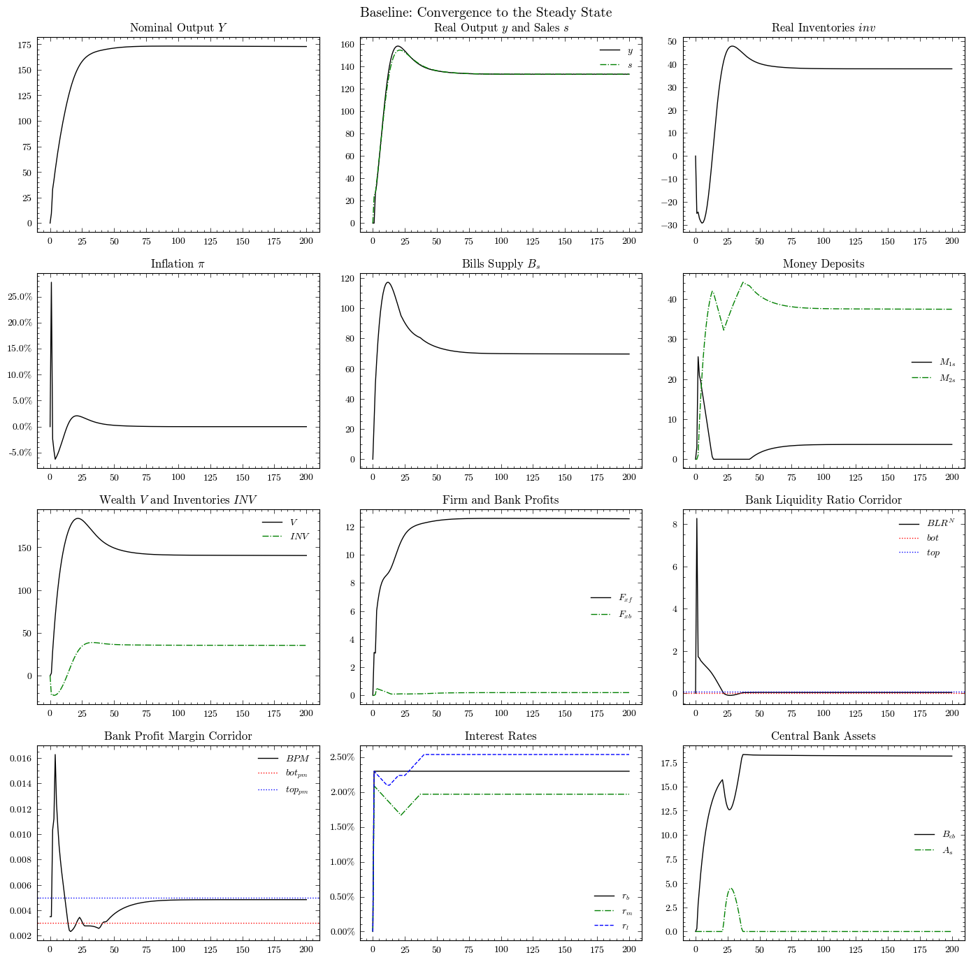
First, we run the model without any shocks to see the convergence to the steady state.

params = ParametersGL06INSOUT()
params.hyper["timesteps"] = 200
params.hyper["scenario_trigger"] = 100
model = GL06INSOUT(parameters=params)
model.simulate()
output = model.variables.to_pandas()

model.variables.check_health(tolerance=1e-3)

True

Convergence to the Steady State

In the steady state with constant exogenous rates, inflation converges to zero, real variables stabilize, and all stock-flow norms reach constant values.

fig, axs = plt.subplots(ncols=3, nrows=4, figsize=(14, 14))

axs[0, 0].plot(output.index, output["NominalOutput"], "k")
axs[0, 0].set_title("Nominal Output $Y$")

axs[0, 1].plot(output.index, output["RealOutput"], "k", label="$y$")
axs[0, 1].plot(output.index, output["RealSales"], "g-.", label="$s$")
axs[0, 1].set_title("Real Output $y$ and Sales $s$")
axs[0, 1].legend(frameon=False)

axs[0, 2].plot(output.index, output["RealInventories"], "k")
axs[0, 2].set_title("Real Inventories $inv$")

axs[1, 0].plot(output.index, output["InflationRate"], "k")
axs[1, 0].set_title(r"Inflation $\pi$")
axs[1, 0].yaxis.set_major_formatter(PercentFormatter(1))

axs[1, 1].plot(output.index, output["BillsSupply"], "k")
axs[1, 1].set_title("Bills Supply $B_s$")

axs[1, 2].plot(output.index, output["M1Supply"], "k", label="$M_{1s}$")
axs[1, 2].plot(output.index, output["M2Supply"], "g-.", label="$M_{2s}$")
axs[1, 2].set_title("Money Deposits")
axs[1, 2].legend(frameon=False)

axs[2, 0].plot(output.index, output["NominalWealth"], "k", label="$V$")
axs[2, 0].plot(output.index, output["NominalInventories"], "g-.", label="$INV$")
axs[2, 0].set_title("Wealth $V$ and Inventories $INV$")
axs[2, 0].legend(frameon=False)

axs[2, 1].plot(output.index, output["FirmProfits"], "k", label="$F_{xf}$")
axs[2, 1].plot(output.index, output["BankProfits"], "g-.", label="$F_{xb}$")
axs[2, 1].set_title("Firm and Bank Profits")
axs[2, 1].legend(frameon=False)

axs[2, 2].plot(
    output.index, output["BankLiquidityRatioTentative"], "k", label="$BLR^N$"
)
axs[2, 2].axhline(y=params["BankLiquidityFloor"], color="r", ls=":", label="$bot$")
axs[2, 2].axhline(y=params["BankLiquidityCeiling"], color="b", ls=":", label="$top$")
axs[2, 2].set_title("Bank Liquidity Ratio Corridor")
axs[2, 2].legend(frameon=False)

axs[3, 0].plot(output.index, output["BankProfitMargin"], "k", label="$BPM$")
axs[3, 0].axhline(y=params["BankProfitFloor"], color="r", ls=":", label="$bot_{pm}$")
axs[3, 0].axhline(y=params["BankProfitCeiling"], color="b", ls=":", label="$top_{pm}$")
axs[3, 0].set_title("Bank Profit Margin Corridor")
axs[3, 0].legend(frameon=False)

axs[3, 1].plot(output.index, output["BillRate"], "k", label="$r_b$")
axs[3, 1].plot(output.index, output["DepositRate"], "g-.", label="$r_m$")
axs[3, 1].plot(output.index, output["LoanRate"], "b--", label="$r_l$")
axs[3, 1].set_title("Interest Rates")
axs[3, 1].yaxis.set_major_formatter(PercentFormatter(1))
axs[3, 1].legend(frameon=False)

axs[3, 2].plot(output.index, output["BillsCentralBank"], "k", label="$B_{cb}$")
axs[3, 2].plot(output.index, output["AdvancesSupply"], "g-.", label="$A_s$")
axs[3, 2].set_title("Central Bank Assets")
axs[3, 2].legend(frameon=False)

fig.suptitle("Baseline: Convergence to the Steady State", fontsize=14)
plt.tight_layout()
plt.show()

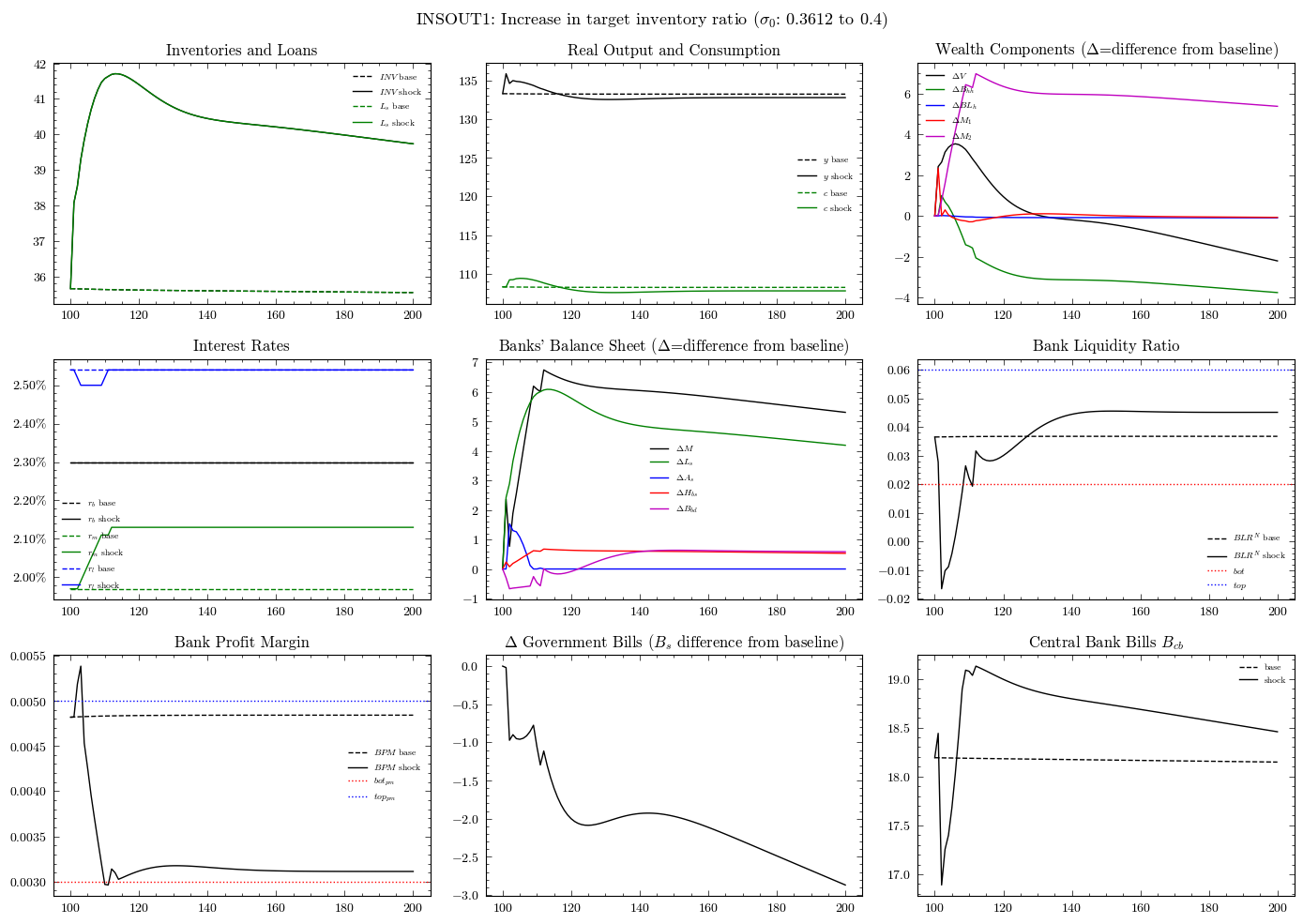
Perturbation 1: Increase in Target Inventory Ratio (INSOUT1)

An increase in \(\sigma_0\) from 0.3612 to 0.4. Firms desire larger inventory buffers, which raises inventory investment, loan demand, and bank lending.

scenarios = ScenariosGL06INSOUT(parameters=params)
sc1 = scenarios.get_scenario_index("Scenario.1: Higher target inventory ratio")
model1 = GL06INSOUT(parameters=params, scenarios=scenarios)
model1.simulate(scenario=sc1)
out1 = model1.variables.to_pandas()

trigger = params["scenario_trigger"]
sl = slice(trigger, None)

fig, axs = plt.subplots(ncols=3, nrows=3, figsize=(14, 10))

# Inventories and Loans
axs[0, 0].plot(
    output.loc[sl].index,
    output.loc[sl, "NominalInventories"],
    "k--",
    label="$INV$ base",
)
axs[0, 0].plot(
    out1.loc[sl].index, out1.loc[sl, "NominalInventories"], "k-", label="$INV$ shock"
)
axs[0, 0].plot(
    output.loc[sl].index, output.loc[sl, "LoansSupply"], "g--", label="$L_s$ base"
)
axs[0, 0].plot(
    out1.loc[sl].index, out1.loc[sl, "LoansSupply"], "g-", label="$L_s$ shock"
)
axs[0, 0].set_title("Inventories and Loans")
axs[0, 0].legend(frameon=False, fontsize=7)

# Real output and consumption
axs[0, 1].plot(
    output.loc[sl].index, output.loc[sl, "RealOutput"], "k--", label="$y$ base"
)
axs[0, 1].plot(out1.loc[sl].index, out1.loc[sl, "RealOutput"], "k-", label="$y$ shock")
axs[0, 1].plot(
    output.loc[sl].index, output.loc[sl, "RealConsumption"], "g--", label="$c$ base"
)
axs[0, 1].plot(
    out1.loc[sl].index, out1.loc[sl, "RealConsumption"], "g-", label="$c$ shock"
)
axs[0, 1].set_title("Real Output and Consumption")
axs[0, 1].legend(frameon=False, fontsize=7)

# Wealth components (delta from baseline)
dV = out1.loc[sl, "NominalWealth"] - output.loc[sl, "NominalWealth"]
dBhh = out1.loc[sl, "BillsHousehold"] - output.loc[sl, "BillsHousehold"]
dBLh = out1.loc[sl, "BondsHousehold"] - output.loc[sl, "BondsHousehold"]
dM1 = out1.loc[sl, "M1Supply"] - output.loc[sl, "M1Supply"]
dM2 = out1.loc[sl, "M2Supply"] - output.loc[sl, "M2Supply"]
axs[0, 2].plot(dV.index, dV, "k-", label=r"$\Delta V$")
axs[0, 2].plot(dBhh.index, dBhh, "g-", label=r"$\Delta B_{hh}$")
axs[0, 2].plot(dBLh.index, dBLh, "b-", label=r"$\Delta BL_h$")
axs[0, 2].plot(dM1.index, dM1, "r-", label=r"$\Delta M_{1}$")
axs[0, 2].plot(dM2.index, dM2, "m-", label=r"$\Delta M_{2}$")
axs[0, 2].set_title(r"Wealth Components ($\Delta$=difference from baseline)")
axs[0, 2].legend(frameon=False, fontsize=7)

# Interest rates
axs[1, 0].plot(
    output.loc[sl].index, output.loc[sl, "BillRate"], "k--", label="$r_b$ base"
)
axs[1, 0].plot(out1.loc[sl].index, out1.loc[sl, "BillRate"], "k-", label="$r_b$ shock")
axs[1, 0].plot(
    output.loc[sl].index, output.loc[sl, "DepositRate"], "g--", label="$r_m$ base"
)
axs[1, 0].plot(
    out1.loc[sl].index, out1.loc[sl, "DepositRate"], "g-", label="$r_m$ shock"
)
axs[1, 0].plot(
    output.loc[sl].index, output.loc[sl, "LoanRate"], "b--", label="$r_l$ base"
)
axs[1, 0].plot(out1.loc[sl].index, out1.loc[sl, "LoanRate"], "b-", label="$r_l$ shock")
axs[1, 0].set_title("Interest Rates")
axs[1, 0].yaxis.set_major_formatter(PercentFormatter(1))
axs[1, 0].legend(frameon=False, fontsize=7)

# Banks' balance sheet (delta from baseline)
dM_tot = (out1.loc[sl, "M1Supply"] + out1.loc[sl, "M2Supply"]) - (
    output.loc[sl, "M1Supply"] + output.loc[sl, "M2Supply"]
)
dLs = out1.loc[sl, "LoansSupply"] - output.loc[sl, "LoansSupply"]
dAs = out1.loc[sl, "AdvancesSupply"] - output.loc[sl, "AdvancesSupply"]
dHbs = out1.loc[sl, "CashBanksSupply"] - output.loc[sl, "CashBanksSupply"]
dBbd = out1.loc[sl, "BillsBank"] - output.loc[sl, "BillsBank"]
axs[1, 1].plot(dM_tot.index, dM_tot, "k-", label=r"$\Delta M$")
axs[1, 1].plot(dLs.index, dLs, "g-", label=r"$\Delta L_s$")
axs[1, 1].plot(dAs.index, dAs, "b-", label=r"$\Delta A_s$")
axs[1, 1].plot(dHbs.index, dHbs, "r-", label=r"$\Delta H_{bs}$")
axs[1, 1].plot(dBbd.index, dBbd, "m-", label=r"$\Delta B_{bd}$")
axs[1, 1].set_title(r"Banks' Balance Sheet ($\Delta$=difference from baseline)")
axs[1, 1].legend(frameon=False, fontsize=7)

# Bank liquidity ratio corridor
axs[1, 2].plot(
    output.loc[sl].index,
    output.loc[sl, "BankLiquidityRatioTentative"],
    "k--",
    label="$BLR^N$ base",
)
axs[1, 2].plot(
    out1.loc[sl].index,
    out1.loc[sl, "BankLiquidityRatioTentative"],
    "k-",
    label="$BLR^N$ shock",
)
axs[1, 2].axhline(y=params["BankLiquidityFloor"], color="r", ls=":", label="$bot$")
axs[1, 2].axhline(y=params["BankLiquidityCeiling"], color="b", ls=":", label="$top$")
axs[1, 2].set_title("Bank Liquidity Ratio")
axs[1, 2].legend(frameon=False, fontsize=7)

# Bank profit margin corridor
axs[2, 0].plot(
    output.loc[sl].index, output.loc[sl, "BankProfitMargin"], "k--", label="$BPM$ base"
)
axs[2, 0].plot(
    out1.loc[sl].index, out1.loc[sl, "BankProfitMargin"], "k-", label="$BPM$ shock"
)
axs[2, 0].axhline(y=params["BankProfitFloor"], color="r", ls=":", label="$bot_{pm}$")
axs[2, 0].axhline(y=params["BankProfitCeiling"], color="b", ls=":", label="$top_{pm}$")
axs[2, 0].set_title("Bank Profit Margin")
axs[2, 0].legend(frameon=False, fontsize=7)

# Government bills change
dGb = out1.loc[sl, "BillsSupply"] - output.loc[sl, "BillsSupply"]
axs[2, 1].plot(dGb.index, dGb, "k-")
axs[2, 1].set_title(r"$\Delta$ Government Bills ($B_s$ difference from baseline)")

# Central bank bills
axs[2, 2].plot(
    output.loc[sl].index, output.loc[sl, "BillsCentralBank"], "k--", label="base"
)
axs[2, 2].plot(
    out1.loc[sl].index, out1.loc[sl, "BillsCentralBank"], "k-", label="shock"
)
axs[2, 2].set_title("Central Bank Bills $B_{cb}$")
axs[2, 2].legend(frameon=False, fontsize=7)

fig.suptitle(
    r"INSOUT1: Increase in target inventory ratio ($\sigma_0$: 0.3612 to 0.4)",
    fontsize=13,
)
plt.tight_layout()
plt.show()

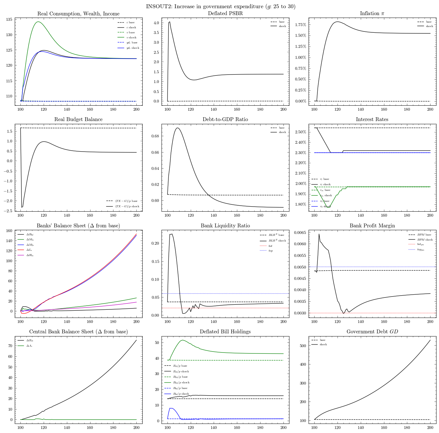
Perturbation 2: Increase in Government Expenditure (INSOUT2)

An increase in real government spending from \(g = 25\) to \(g = 30\). This is the standard Keynesian fiscal expansion.

scenarios = ScenariosGL06INSOUT(parameters=params)
sc2 = scenarios.get_scenario_index("Scenario.2: Higher government spending")
model2 = GL06INSOUT(parameters=params, scenarios=scenarios)
model2.simulate(scenario=sc2)
out2 = model2.variables.to_pandas()

trigger = params["scenario_trigger"]
sl = slice(trigger, None)

fig, axs = plt.subplots(ncols=3, nrows=4, figsize=(14, 14))

# Real consumption, wealth, and income
p_base = output.loc[sl, "PriceLevel"].values
p_shock = out2.loc[sl, "PriceLevel"].values
axs[0, 0].plot(
    output.loc[sl].index, output.loc[sl, "RealConsumption"], "k--", label="$c$ base"
)
axs[0, 0].plot(
    out2.loc[sl].index, out2.loc[sl, "RealConsumption"], "k-", label="$c$ shock"
)
axs[0, 0].plot(
    output.loc[sl].index,
    output.loc[sl, "NominalWealth"].values / p_base,
    "g--",
    label="$v$ base",
)
axs[0, 0].plot(
    out2.loc[sl].index,
    out2.loc[sl, "NominalWealth"].values / p_shock,
    "g-",
    label="$v$ shock",
)
axs[0, 0].plot(
    output.loc[sl].index,
    output.loc[sl, "RealRegularDisposableIncome"],
    "b--",
    label="$yd_r$ base",
)
axs[0, 0].plot(
    out2.loc[sl].index,
    out2.loc[sl, "RealRegularDisposableIncome"],
    "b-",
    label="$yd_r$ shock",
)
axs[0, 0].set_title("Real Consumption, Wealth, Income")
axs[0, 0].legend(frameon=False, fontsize=7)

# Deflated PSBR
axs[0, 1].plot(
    output.loc[sl].index,
    output.loc[sl, "PublicSectorBorrowingRequirement"].values / p_base,
    "k--",
    label="base",
)
axs[0, 1].plot(
    out2.loc[sl].index,
    out2.loc[sl, "PublicSectorBorrowingRequirement"].values / p_shock,
    "k-",
    label="shock",
)
axs[0, 1].set_title("Deflated PSBR")
axs[0, 1].legend(frameon=False, fontsize=7)

# Inflation
axs[0, 2].plot(
    output.loc[sl].index, output.loc[sl, "InflationRate"], "k--", label="base"
)
axs[0, 2].plot(out2.loc[sl].index, out2.loc[sl, "InflationRate"], "k-", label="shock")
axs[0, 2].set_title(r"Inflation $\pi$")
axs[0, 2].yaxis.set_major_formatter(PercentFormatter(1))
axs[0, 2].legend(frameon=False, fontsize=7)

# Real budget balance
budget_base = (
    output.loc[sl, "Taxes"].values - output.loc[sl, "GovernmentSpending"].values
) / p_base
budget_shock = (
    out2.loc[sl, "Taxes"].values - out2.loc[sl, "GovernmentSpending"].values
) / p_shock
axs[1, 0].plot(output.loc[sl].index, budget_base, "k--", label="$(TX-G)/p$ base")
axs[1, 0].plot(out2.loc[sl].index, budget_shock, "k-", label="$(TX-G)/p$ shock")
axs[1, 0].set_title("Real Budget Balance")
axs[1, 0].legend(frameon=False, fontsize=7)

# Debt-to-GDP ratio
byr_base = (
    output.loc[sl, "GovernmentDebt"].values / output.loc[sl, "NominalOutput"].values
)
byr_shock = out2.loc[sl, "GovernmentDebt"].values / out2.loc[sl, "NominalOutput"].values
axs[1, 1].plot(output.loc[sl].index, byr_base, "k--", label="base")
axs[1, 1].plot(out2.loc[sl].index, byr_shock, "k-", label="shock")
axs[1, 1].set_title("Debt-to-GDP Ratio")
axs[1, 1].legend(frameon=False, fontsize=7)

# Interest rates
axs[1, 2].plot(
    output.loc[sl].index, output.loc[sl, "LoanRate"], "k--", label="$r_l$ base"
)
axs[1, 2].plot(out2.loc[sl].index, out2.loc[sl, "LoanRate"], "k-", label="$r_l$ shock")
axs[1, 2].plot(
    output.loc[sl].index, output.loc[sl, "DepositRate"], "g--", label="$r_m$ base"
)
axs[1, 2].plot(
    out2.loc[sl].index, out2.loc[sl, "DepositRate"], "g-", label="$r_m$ shock"
)
axs[1, 2].plot(
    output.loc[sl].index, output.loc[sl, "BillRate"], "b--", label="$r_b$ base"
)
axs[1, 2].plot(out2.loc[sl].index, out2.loc[sl, "BillRate"], "b-", label="$r_b$ shock")
axs[1, 2].set_title("Interest Rates")
axs[1, 2].yaxis.set_major_formatter(PercentFormatter(1))
axs[1, 2].legend(frameon=False, fontsize=7)

# Banks' balance sheet (delta from baseline)
dBbd = out2.loc[sl, "BillsBank"] - output.loc[sl, "BillsBank"]
dM1s = out2.loc[sl, "M1Supply"] - output.loc[sl, "M1Supply"]
dM2s = out2.loc[sl, "M2Supply"] - output.loc[sl, "M2Supply"]
dLs = out2.loc[sl, "LoansSupply"] - output.loc[sl, "LoansSupply"]
dHbs = out2.loc[sl, "CashBanksSupply"] - output.loc[sl, "CashBanksSupply"]
axs[2, 0].plot(dBbd.index, dBbd, "k-", label=r"$\Delta B_{bd}$")
axs[2, 0].plot(dM1s.index, dM1s, "g-", label=r"$\Delta M_{1s}$")
axs[2, 0].plot(dM2s.index, dM2s, "b-", label=r"$\Delta M_{2s}$")
axs[2, 0].plot(dLs.index, dLs, "r-", label=r"$\Delta L_s$")
axs[2, 0].plot(dHbs.index, dHbs, "m-", label=r"$\Delta H_{bs}$")
axs[2, 0].set_title(r"Banks' Balance Sheet ($\Delta$ from base)")
axs[2, 0].legend(frameon=False, fontsize=7)

# Bank liquidity ratio corridor
axs[2, 1].plot(
    output.loc[sl].index,
    output.loc[sl, "BankLiquidityRatioTentative"],
    "k--",
    label="$BLR^N$ base",
)
axs[2, 1].plot(
    out2.loc[sl].index,
    out2.loc[sl, "BankLiquidityRatioTentative"],
    "k-",
    label="$BLR^N$ shock",
)
axs[2, 1].axhline(y=params["BankLiquidityFloor"], color="r", ls=":", label="$bot$")
axs[2, 1].axhline(y=params["BankLiquidityCeiling"], color="b", ls=":", label="$top$")
axs[2, 1].set_title("Bank Liquidity Ratio")
axs[2, 1].legend(frameon=False, fontsize=7)

# Bank profit margin corridor
axs[2, 2].plot(
    output.loc[sl].index, output.loc[sl, "BankProfitMargin"], "k--", label="$BPM$ base"
)
axs[2, 2].plot(
    out2.loc[sl].index, out2.loc[sl, "BankProfitMargin"], "k-", label="$BPM$ shock"
)
axs[2, 2].axhline(y=params["BankProfitFloor"], color="r", ls=":", label="$bot_{pm}$")
axs[2, 2].axhline(y=params["BankProfitCeiling"], color="b", ls=":", label="$top_{pm}$")
axs[2, 2].set_title("Bank Profit Margin")
axs[2, 2].legend(frameon=False, fontsize=7)

# Central bank balance sheet (delta)
dAs = out2.loc[sl, "AdvancesSupply"] - output.loc[sl, "AdvancesSupply"]
dBcb = out2.loc[sl, "BillsCentralBank"] - output.loc[sl, "BillsCentralBank"]
axs[3, 0].plot(dBcb.index, dBcb, "k-", label=r"$\Delta B_{cb}$")
axs[3, 0].plot(dAs.index, dAs, "g-", label=r"$\Delta A_s$")
axs[3, 0].set_title(r"Central Bank Balance Sheet ($\Delta$ from base)")
axs[3, 0].legend(frameon=False, fontsize=7)

# Deflated bill holdings
axs[3, 1].plot(
    output.loc[sl].index,
    output.loc[sl, "BillsCentralBank"].values / p_base,
    "k--",
    label="$B_{cb}/p$ base",
)
axs[3, 1].plot(
    out2.loc[sl].index,
    out2.loc[sl, "BillsCentralBank"].values / p_shock,
    "k-",
    label="$B_{cb}/p$ shock",
)
axs[3, 1].plot(
    output.loc[sl].index,
    output.loc[sl, "BillsHousehold"].values / p_base,
    "g--",
    label="$B_{hh}/p$ base",
)
axs[3, 1].plot(
    out2.loc[sl].index,
    out2.loc[sl, "BillsHousehold"].values / p_shock,
    "g-",
    label="$B_{hh}/p$ shock",
)
axs[3, 1].plot(
    output.loc[sl].index,
    output.loc[sl, "BillsBank"].values / p_base,
    "b--",
    label="$B_{bd}/p$ base",
)
axs[3, 1].plot(
    out2.loc[sl].index,
    out2.loc[sl, "BillsBank"].values / p_shock,
    "b-",
    label="$B_{bd}/p$ shock",
)
axs[3, 1].set_title("Deflated Bill Holdings")
axs[3, 1].legend(frameon=False, fontsize=7)

# Government debt
axs[3, 2].plot(
    output.loc[sl].index, output.loc[sl, "GovernmentDebt"], "k--", label="base"
)
axs[3, 2].plot(out2.loc[sl].index, out2.loc[sl, "GovernmentDebt"], "k-", label="shock")
axs[3, 2].set_title("Government Debt $GD$")
axs[3, 2].legend(frameon=False, fontsize=7)

fig.suptitle("INSOUT2: Increase in government expenditure ($g$: 25 to 30)", fontsize=13)
plt.tight_layout()
plt.show()

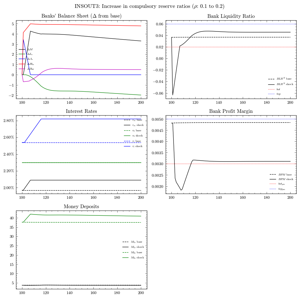
Perturbation 3: Increase in Compulsory Reserve Ratios (INSOUT3)

An increase in reserve ratios from \(\rho_1 = \rho_2 = 0.1\) to \(\rho_1 = \rho_2 = 0.2\).

scenarios = ScenariosGL06INSOUT(parameters=params)
sc3 = scenarios.get_scenario_index("Scenario.3: Higher reserve requirements")
model3 = GL06INSOUT(parameters=params, scenarios=scenarios)
model3.simulate(scenario=sc3)
out3 = model3.variables.to_pandas()

trigger = params["scenario_trigger"]
sl = slice(trigger, None)

fig, axs = plt.subplots(ncols=2, nrows=3, figsize=(10, 10))

# Banks' balance sheet (delta from baseline)
dM = (out3.loc[sl, "M1Supply"] + out3.loc[sl, "M2Supply"]) - (
    output.loc[sl, "M1Supply"] + output.loc[sl, "M2Supply"]
)
dLs = out3.loc[sl, "LoansSupply"] - output.loc[sl, "LoansSupply"]
dAs = out3.loc[sl, "AdvancesSupply"] - output.loc[sl, "AdvancesSupply"]
dHbs = out3.loc[sl, "CashBanksSupply"] - output.loc[sl, "CashBanksSupply"]
dBbd = out3.loc[sl, "BillsBank"] - output.loc[sl, "BillsBank"]
axs[0, 0].plot(dM.index, dM, "k-", label=r"$\Delta M$")
axs[0, 0].plot(dLs.index, dLs, "g-", label=r"$\Delta L_s$")
axs[0, 0].plot(dAs.index, dAs, "b-", label=r"$\Delta A_s$")
axs[0, 0].plot(dHbs.index, dHbs, "r-", label=r"$\Delta H_{bs}$")
axs[0, 0].plot(dBbd.index, dBbd, "m-", label=r"$\Delta B_{bd}$")
axs[0, 0].set_title(r"Banks' Balance Sheet ($\Delta$ from base)")
axs[0, 0].legend(frameon=False, fontsize=7)

# Bank liquidity ratio corridor
axs[0, 1].plot(
    output.loc[sl].index,
    output.loc[sl, "BankLiquidityRatioTentative"],
    "k--",
    label="$BLR^N$ base",
)
axs[0, 1].plot(
    out3.loc[sl].index,
    out3.loc[sl, "BankLiquidityRatioTentative"],
    "k-",
    label="$BLR^N$ shock",
)
axs[0, 1].axhline(y=params["BankLiquidityFloor"], color="r", ls=":", label="$bot$")
axs[0, 1].axhline(y=params["BankLiquidityCeiling"], color="b", ls=":", label="$top$")
axs[0, 1].set_title("Bank Liquidity Ratio")
axs[0, 1].legend(frameon=False, fontsize=7)

# Interest rates
axs[1, 0].plot(
    output.loc[sl].index, output.loc[sl, "DepositRate"], "k--", label="$r_m$ base"
)
axs[1, 0].plot(
    out3.loc[sl].index, out3.loc[sl, "DepositRate"], "k-", label="$r_m$ shock"
)
axs[1, 0].plot(
    output.loc[sl].index, output.loc[sl, "BillRate"], "g--", label="$r_b$ base"
)
axs[1, 0].plot(out3.loc[sl].index, out3.loc[sl, "BillRate"], "g-", label="$r_b$ shock")
axs[1, 0].plot(
    output.loc[sl].index, output.loc[sl, "LoanRate"], "b--", label="$r_l$ base"
)
axs[1, 0].plot(out3.loc[sl].index, out3.loc[sl, "LoanRate"], "b-", label="$r_l$ shock")
axs[1, 0].set_title("Interest Rates")
axs[1, 0].yaxis.set_major_formatter(PercentFormatter(1))
axs[1, 0].legend(frameon=False, fontsize=7)

# Bank profit margin corridor
axs[1, 1].plot(
    output.loc[sl].index, output.loc[sl, "BankProfitMargin"], "k--", label="$BPM$ base"
)
axs[1, 1].plot(
    out3.loc[sl].index, out3.loc[sl, "BankProfitMargin"], "k-", label="$BPM$ shock"
)
axs[1, 1].axhline(y=params["BankProfitFloor"], color="r", ls=":", label="$bot_{pm}$")
axs[1, 1].axhline(y=params["BankProfitCeiling"], color="b", ls=":", label="$top_{pm}$")
axs[1, 1].set_title("Bank Profit Margin")
axs[1, 1].legend(frameon=False, fontsize=7)

# Money deposits
axs[2, 0].plot(
    output.loc[sl].index, output.loc[sl, "M1Supply"], "k--", label="$M_{1s}$ base"
)
axs[2, 0].plot(
    out3.loc[sl].index, out3.loc[sl, "M1Supply"], "k-", label="$M_{1s}$ shock"
)
axs[2, 0].plot(
    output.loc[sl].index, output.loc[sl, "M2Supply"], "g--", label="$M_{2s}$ base"
)
axs[2, 0].plot(
    out3.loc[sl].index, out3.loc[sl, "M2Supply"], "g-", label="$M_{2s}$ shock"
)
axs[2, 0].set_title("Money Deposits")
axs[2, 0].legend(frameon=False, fontsize=7)

axs[2, 1].axis("off")

fig.suptitle(
    r"INSOUT3: Increase in compulsory reserve ratios ($\rho$: 0.1 to 0.2)", fontsize=13
)
plt.tight_layout()
plt.show()

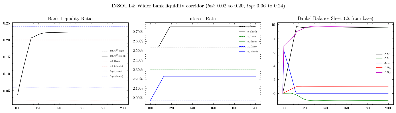
Perturbation 4: Increase in Acceptable Bank Liquidity Ratio (INSOUT4)

An increase in the liquidity corridor from \(bot = 0.02, top = 0.06\) to \(bot = 0.20, top = 0.24\).

scenarios = ScenariosGL06INSOUT(parameters=params)
sc4 = scenarios.get_scenario_index("Scenario.4: Wider liquidity corridor")
model4 = GL06INSOUT(parameters=params, scenarios=scenarios)
model4.simulate(scenario=sc4)
out4 = model4.variables.to_pandas()

trigger = params["scenario_trigger"]
sl = slice(trigger, None)

fig, axs = plt.subplots(ncols=3, nrows=1, figsize=(14, 4))

# Bank liquidity ratio corridor
axs[0].plot(
    output.loc[sl].index,
    output.loc[sl, "BankLiquidityRatioTentative"],
    "k--",
    label="$BLR^N$ base",
)
axs[0].plot(
    out4.loc[sl].index,
    out4.loc[sl, "BankLiquidityRatioTentative"],
    "k-",
    label="$BLR^N$ shock",
)
axs[0].axhline(
    y=params["BankLiquidityFloor"], color="r", ls=":", alpha=0.5, label="$bot$ (base)"
)
axs[0].axhline(y=0.20, color="r", ls="--", alpha=0.5, label="$bot$ (shock)")
axs[0].axhline(
    y=params["BankLiquidityCeiling"], color="b", ls=":", alpha=0.5, label="$top$ (base)"
)
axs[0].axhline(y=0.24, color="b", ls="--", alpha=0.5, label="$top$ (shock)")
axs[0].set_title("Bank Liquidity Ratio")
axs[0].legend(frameon=False, fontsize=7)

# Interest rates
axs[1].plot(output.loc[sl].index, output.loc[sl, "LoanRate"], "k--", label="$r_l$ base")
axs[1].plot(out4.loc[sl].index, out4.loc[sl, "LoanRate"], "k-", label="$r_l$ shock")
axs[1].plot(output.loc[sl].index, output.loc[sl, "BillRate"], "g--", label="$r_b$ base")
axs[1].plot(out4.loc[sl].index, out4.loc[sl, "BillRate"], "g-", label="$r_b$ shock")
axs[1].plot(
    output.loc[sl].index, output.loc[sl, "DepositRate"], "b--", label="$r_m$ base"
)
axs[1].plot(out4.loc[sl].index, out4.loc[sl, "DepositRate"], "b-", label="$r_m$ shock")
axs[1].set_title("Interest Rates")
axs[1].yaxis.set_major_formatter(PercentFormatter(1))
axs[1].legend(frameon=False, fontsize=7)

# Banks' balance sheet (delta from baseline)
dM = (out4.loc[sl, "M1Supply"] + out4.loc[sl, "M2Supply"]) - (
    output.loc[sl, "M1Supply"] + output.loc[sl, "M2Supply"]
)
dLs = out4.loc[sl, "LoansSupply"] - output.loc[sl, "LoansSupply"]
dAs = out4.loc[sl, "AdvancesSupply"] - output.loc[sl, "AdvancesSupply"]
dHbs = out4.loc[sl, "CashBanksSupply"] - output.loc[sl, "CashBanksSupply"]
dBbd = out4.loc[sl, "BillsBank"] - output.loc[sl, "BillsBank"]
axs[2].plot(dM.index, dM, "k-", label=r"$\Delta M$")
axs[2].plot(dLs.index, dLs, "g-", label=r"$\Delta L_s$")
axs[2].plot(dAs.index, dAs, "b-", label=r"$\Delta A_s$")
axs[2].plot(dHbs.index, dHbs, "r-", label=r"$\Delta H_{bs}$")
axs[2].plot(dBbd.index, dBbd, "m-", label=r"$\Delta B_{bd}$")
axs[2].set_title(r"Banks' Balance Sheet ($\Delta$ from base)")
axs[2].legend(frameon=False, fontsize=7)

fig.suptitle(
    "INSOUT4: Wider bank liquidity corridor ($bot$: 0.02 to 0.20, $top$: 0.06 to 0.24)",
    fontsize=13,
)
plt.tight_layout()
plt.show()

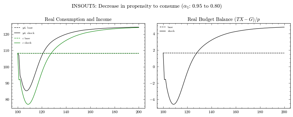
Perturbation 5: Decrease in Propensity to Consume (INSOUT5)

A decrease in \(\alpha_1\) from 0.95 to 0.80. The paradox-of-thrift experiment.

scenarios = ScenariosGL06INSOUT(parameters=params)
sc5 = scenarios.get_scenario_index("Scenario.5: Lower consumption propensity")
model5 = GL06INSOUT(parameters=params, scenarios=scenarios)
model5.simulate(scenario=sc5)
out5 = model5.variables.to_pandas()

trigger = params["scenario_trigger"]
sl = slice(trigger, None)

fig, axs = plt.subplots(ncols=2, nrows=1, figsize=(10, 4))

# Real consumption and income
axs[0].plot(
    output.loc[sl].index,
    output.loc[sl, "RealRegularDisposableIncome"],
    "k--",
    label="$yd_r$ base",
)
axs[0].plot(
    out5.loc[sl].index,
    out5.loc[sl, "RealRegularDisposableIncome"],
    "k-",
    label="$yd_r$ shock",
)
axs[0].plot(
    output.loc[sl].index, output.loc[sl, "RealConsumption"], "g--", label="$c$ base"
)
axs[0].plot(
    out5.loc[sl].index, out5.loc[sl, "RealConsumption"], "g-", label="$c$ shock"
)
axs[0].set_title("Real Consumption and Income")
axs[0].legend(frameon=False, fontsize=7)

# Real budget balance
budget_base = (
    output.loc[sl, "Taxes"].values - output.loc[sl, "GovernmentSpending"].values
) / output.loc[sl, "PriceLevel"].values
budget_shock = (
    out5.loc[sl, "Taxes"].values - out5.loc[sl, "GovernmentSpending"].values
) / out5.loc[sl, "PriceLevel"].values
axs[1].plot(output.loc[sl].index, budget_base, "k--", label="base")
axs[1].plot(out5.loc[sl].index, budget_shock, "k-", label="shock")
axs[1].set_title("Real Budget Balance $(TX - G)/p$")
axs[1].legend(frameon=False, fontsize=7)

fig.suptitle(
    r"INSOUT5: Decrease in propensity to consume ($\alpha_1$: 0.95 to 0.80)",
    fontsize=13,
)
plt.tight_layout()
plt.show()

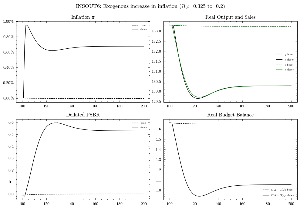
Perturbation 6: Exogenous Increase in Inflation via Wage Target (INSOUT6)

An increase in the real wage target constant from \(\Omega_0 = -0.32549\) to \(\Omega_0 = -0.2\). Workers push for a higher real wage, triggering a wage-price spiral.

scenarios = ScenariosGL06INSOUT(parameters=params)
sc6 = scenarios.get_scenario_index("Scenario.6: Higher real wage target")
model6 = GL06INSOUT(parameters=params, scenarios=scenarios)
model6.simulate(scenario=sc6)
out6 = model6.variables.to_pandas()

trigger = params["scenario_trigger"]
sl = slice(trigger, None)

fig, axs = plt.subplots(ncols=2, nrows=2, figsize=(10, 7))

# Inflation
axs[0, 0].plot(
    output.loc[sl].index, output.loc[sl, "InflationRate"], "k--", label="base"
)
axs[0, 0].plot(out6.loc[sl].index, out6.loc[sl, "InflationRate"], "k-", label="shock")
axs[0, 0].set_title(r"Inflation $\pi$")
axs[0, 0].yaxis.set_major_formatter(PercentFormatter(1))
axs[0, 0].legend(frameon=False, fontsize=7)

# Real output and sales
axs[0, 1].plot(
    output.loc[sl].index, output.loc[sl, "RealOutput"], "k--", label="$y$ base"
)
axs[0, 1].plot(out6.loc[sl].index, out6.loc[sl, "RealOutput"], "k-", label="$y$ shock")
axs[0, 1].plot(
    output.loc[sl].index, output.loc[sl, "RealSales"], "g--", label="$s$ base"
)
axs[0, 1].plot(out6.loc[sl].index, out6.loc[sl, "RealSales"], "g-", label="$s$ shock")
axs[0, 1].set_title("Real Output and Sales")
axs[0, 1].legend(frameon=False, fontsize=7)

# Deflated PSBR
p_base = output.loc[sl, "PriceLevel"].values
p_shock = out6.loc[sl, "PriceLevel"].values
axs[1, 0].plot(
    output.loc[sl].index,
    output.loc[sl, "PublicSectorBorrowingRequirement"].values / p_base,
    "k--",
    label="base",
)
axs[1, 0].plot(
    out6.loc[sl].index,
    out6.loc[sl, "PublicSectorBorrowingRequirement"].values / p_shock,
    "k-",
    label="shock",
)
axs[1, 0].set_title("Deflated PSBR")
axs[1, 0].legend(frameon=False, fontsize=7)

# Real budget balance
budget_base = (
    output.loc[sl, "Taxes"].values - output.loc[sl, "GovernmentSpending"].values
) / p_base
budget_shock = (
    out6.loc[sl, "Taxes"].values - out6.loc[sl, "GovernmentSpending"].values
) / p_shock
axs[1, 1].plot(output.loc[sl].index, budget_base, "k--", label="$(TX-G)/p$ base")
axs[1, 1].plot(out6.loc[sl].index, budget_shock, "k-", label="$(TX-G)/p$ shock")
axs[1, 1].set_title("Real Budget Balance")
axs[1, 1].legend(frameon=False, fontsize=7)

fig.suptitle(
    r"INSOUT6: Exogenous increase in inflation ($\Omega_0$: -0.325 to -0.2)",
    fontsize=13,
)
plt.tight_layout()
plt.show()

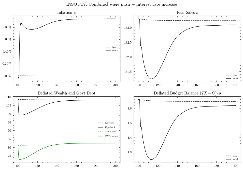
Perturbation 7: Combined Wage Push and Interest Rate Increase (INSOUT7)

A simultaneous wage push (\(\Omega_0\): -0.325 to -0.2) and interest rate increase (\(r_b\): 0.023 to 0.03, \(r_{bl}\): 0.027 to 0.039). This stagflation experiment shows the interaction between cost-push inflation and monetary contraction.

scenarios = ScenariosGL06INSOUT(parameters=params)
sc7 = scenarios.get_scenario_index("Scenario.7: Wage target + rate rise")
model7 = GL06INSOUT(parameters=params, scenarios=scenarios)
model7.simulate(scenario=sc7)
out7 = model7.variables.to_pandas()

trigger = params["scenario_trigger"]
sl = slice(trigger, None)

fig, axs = plt.subplots(ncols=2, nrows=2, figsize=(10, 7))

# Inflation
axs[0, 0].plot(
    output.loc[sl].index, output.loc[sl, "InflationRate"], "k--", label="base"
)
axs[0, 0].plot(out7.loc[sl].index, out7.loc[sl, "InflationRate"], "k-", label="shock")
axs[0, 0].set_title(r"Inflation $\pi$")
axs[0, 0].yaxis.set_major_formatter(PercentFormatter(1))
axs[0, 0].legend(frameon=False, fontsize=7)

# Real sales
axs[0, 1].plot(output.loc[sl].index, output.loc[sl, "RealSales"], "k--", label="base")
axs[0, 1].plot(out7.loc[sl].index, out7.loc[sl, "RealSales"], "k-", label="shock")
axs[0, 1].set_title("Real Sales $s$")
axs[0, 1].legend(frameon=False, fontsize=7)

# Deflated wealth vs government debt
p_base = output.loc[sl, "PriceLevel"].values
p_shock = out7.loc[sl, "PriceLevel"].values
axs[1, 0].plot(
    output.loc[sl].index,
    output.loc[sl, "NominalWealth"].values / p_base,
    "k--",
    label="$V/p$ base",
)
axs[1, 0].plot(
    out7.loc[sl].index,
    out7.loc[sl, "NominalWealth"].values / p_shock,
    "k-",
    label="$V/p$ shock",
)
axs[1, 0].plot(
    output.loc[sl].index,
    output.loc[sl, "GovernmentDebt"].values / p_base,
    "g--",
    label="$GD/p$ base",
)
axs[1, 0].plot(
    out7.loc[sl].index,
    out7.loc[sl, "GovernmentDebt"].values / p_shock,
    "g-",
    label="$GD/p$ shock",
)
axs[1, 0].set_title("Deflated Wealth and Govt Debt")
axs[1, 0].legend(frameon=False, fontsize=7)

# Deflated budget balance
budget_base = (
    output.loc[sl, "Taxes"].values - output.loc[sl, "GovernmentSpending"].values
) / p_base
budget_shock = (
    out7.loc[sl, "Taxes"].values - out7.loc[sl, "GovernmentSpending"].values
) / p_shock
axs[1, 1].plot(output.loc[sl].index, budget_base, "k--", label="base")
axs[1, 1].plot(out7.loc[sl].index, budget_shock, "k-", label="shock")
axs[1, 1].set_title("Deflated Budget Balance $(TX-G)/p$")
axs[1, 1].legend(frameon=False, fontsize=7)

fig.suptitle("INSOUT7: Combined wage push + interest rate increase", fontsize=13)
plt.tight_layout()
plt.show()

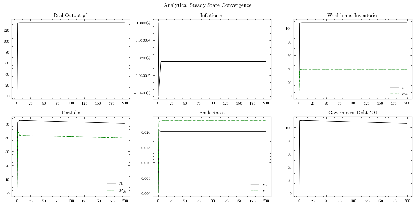
Theoretical Steady State

INSOUT includes an analytical steady-state solver that computes all state variables from parameters alone, without running a long simulation to convergence. The solver derives \(UC/p\) analytically, expresses portfolio quantities as linear functions of \(y^*\), and solves a quadratic equation from GL06 eq. 10.98 to obtain real output. Inflation is determined jointly via Picard iteration on the wage equation.

params_ss = ParametersGL06INSOUT()
params_ss.hyper["timesteps"] = 200
params_ss.hyper["scenario_trigger"] = 100
model_ss = GL06INSOUT(parameters=params_ss)
model_ss.compute_theoretical_steady_state()
ss_output = model_ss.variables.to_pandas()

INFO:root:Computing theoretical steady state. Scenario: 0

The solver converges in approximately 20 outer-loop iterations (for bank rate equilibration). The resulting steady-state values match long-run simulation within 0.2% for the baseline calibration.

fig, axs = plt.subplots(ncols=3, nrows=2, figsize=(14, 7))

axs[0, 0].plot(ss_output.index, ss_output["RealOutput"], "k")
axs[0, 0].set_title("Real Output $y^*$")

axs[0, 1].plot(ss_output.index, ss_output["InflationRate"], "k")
axs[0, 1].set_title(r"Inflation $\pi$")
axs[0, 1].yaxis.set_major_formatter(PercentFormatter(1))

axs[0, 2].plot(ss_output.index, ss_output["RealWealth"], "k", label="$v$")
axs[0, 2].plot(ss_output.index, ss_output["RealInventories"], "g-.", label="$inv$")
axs[0, 2].set_title("Wealth and Inventories")
axs[0, 2].legend(frameon=False)

axs[1, 0].plot(ss_output.index, ss_output["BillsHousehold"], "k", label="$B_h$")
axs[1, 0].plot(ss_output.index, ss_output["M2Household"], "g-.", label="$M_{2h}$")
axs[1, 0].set_title("Portfolio")
axs[1, 0].legend(frameon=False)

axs[1, 1].plot(ss_output.index, ss_output["DepositRate"], "k", label="$r_m$")
axs[1, 1].plot(ss_output.index, ss_output["LoanRate"], "g-.", label="$r_l$")
axs[1, 1].set_title("Bank Rates")
axs[1, 1].legend(frameon=False)

axs[1, 2].plot(ss_output.index, ss_output["GovernmentDebt"], "k")
axs[1, 2].set_title("Government Debt $GD$")

fig.suptitle("Analytical Steady-State Convergence", fontsize=13)
plt.tight_layout()
plt.show()