Model PCEX#
Model PCEX is introduced in chapter 4 of Godley and Lavoie [2006] “Monetary Economics: An Integrated Approach to Credit, Money, Income, Production and Wealth”. In its setup, the model has the same transactions and balance sheet as Model PC (see here), but features expectations on disposable income and wealth.
Module Contents#
As with all MacroStat models, PCEX is divided into Variables, Parameters (fixed constants), Scenarios, and the Behavior (model initialization and steps). The module-level documentation, such as all variables/parameters/scenarios and their notation or the behavioral equations associated with each function of BehaviorPCEX.py can be seen in:
The remainder of this page gives an introduction to the model, notes on how it is implemented in MacroStat and then shows some of the model dynamics by replicating the relevant graphs of Godley and Lavoie (2006).
Model Overview#
Behavioral Equations#
Unlike model PC, model PCEX is built with expectations. Specifically, the household forms expectations of its disposable income \(YD^e\) and its expected wealth \(V^e\). With these two variables, the remaining equations of the model are almost identical to model PC.
National Income
Disposable income is national income and interest earnings minus taxes
Taxes are a fixed share of income
Wealth increases by savings
Consumption is partially out of disposable income and wealth, but now based on expected disposable income
The share of bills in wealth depends on expected wealth and expected disposable income
The share of cash in wealth (6A)
Household cash demand can also be described by the difference between expected wealth and demand for bills
expected wealth depends on expected disposable income
The household’s realized cash holdings then depend on the realisation of household wealth
Where we assume now that the household’s demand for bills is met.
The change in the stock of outstanding government bills (also known as the government’s budget constraint). The first part represents government outlays (direct purchases and interest payments) while the second represents government revenues (taxes and central bank profits)
The change in money circulating
Bills held by the central bank, the central bank purchases all of the bills issued by the government that the households are not willing to buy given the current interest rate. Combined with
gl06_pc_eq409_moneyIssuanceit implies the CB provides cash money on demand. Therefore, the amount of cash in the system is endogeneous and demand-led while the rate on bills is exogenous.
The interest rate is fixed
With the redundant equation being
Now we must still define how the expected disposable income is set, as with model SIMEX, we suppose that it is a simple extrapolation from prior levels (which is self-consistent in a steady state since the economy is not growing here).
Note that in Godley and Lavoie [2006] this is equivalent to Model PCEX1, while Model PCEX actually just assumes a random multiplicative term on the \(YD\) determined by model PC. I do not here model this part, as it is only used as a demonstration in the book.
Transaction Flow Matrix#
Household |
Production |
Government |
CentralBank |
CentralBank |
Total |
|
|---|---|---|---|---|---|---|
Current |
Current |
Current |
Current |
Capital |
||
Consumption Household |
\(-C(t)\) |
\(+C(t)\) |
\(0\) |
|||
Consumption Government |
\(+G(t)\) |
\(-G(t)\) |
\(0\) |
|||
National Income |
\(+Y(t)\) |
\(-Y(t)\) |
\(0\) |
|||
Interest Earned On Bills Household |
\(+r(t-1)\cdot B_h(t-1)\) |
\(-r(t-1)\cdot B_h(t-1)\) |
\(0\) |
|||
Central Bank Profits |
\(+r(t-1)\cdot B_{CB}(t-1)\) |
\(-r(t-1)\cdot B_{CB}(t-1)\) |
\(0\) |
|||
Taxes |
\(-T(t)\) |
\(+T(t)\) |
\(0\) |
|||
Change in Money Stock |
\(+\Delta H_h(t)\) |
\(-\Delta H_{s}(t)\) |
\(0\) |
|||
Change in Bill Stock |
\(+\Delta B_h(t)\) |
\(-\Delta B_s(t)\) |
\(+\Delta B_{CB}(t)\) |
\(0\) |
||
Total |
\(0\) |
\(0\) |
\(0\) |
\(0\) |
\(0\) |
\(0\) |
Balance Sheet Matrix#
Household |
Production |
Government |
CentralBank |
Total |
|
|---|---|---|---|---|---|
Current |
Current |
Current |
Capital |
||
Money Stock |
\(+H_h(t)\) |
\(-H_{s}(t)\) |
0 |
||
Bill Stock |
\(+B_h(t)\) |
\(-B_s(t)\) |
\(+B_{CB}(t)\) |
0 |
|
Wealth |
\(-V(t)\) |
\(+V(t)\) |
0 |
Implementation in MacroStat#
Transposing these eleven equations to the MacroStat framework, we consider that there are:
Three parameters (fixed constants): \(\alpha_1\), \(\alpha_2\), and \(\theta\) (see Parameters)
Two scenario variables : \(G_d(t)\) and \(W(t)\) (see Scenarios)
The remaining tracked series are variables (see Variables)
Model Dynamics#
Preparatory Steps#
%load_ext autoreload
%autoreload 2

import importlib
import logging
import sys

# Import the necessary libraries for plotting
from matplotlib import pyplot as plt
from matplotlib.ticker import PercentFormatter

# Import the MacroStat get_model function
from macrostat.models import get_model

# Custom matplotlib style for the documentation
plt.style.use("../../macrostat.mplstyle")
# We show the logging output in the notebook
importlib.reload(logging)
logging.basicConfig(stream=sys.stdout, level=logging.INFO)
Running the Simulation#
First, we can run the model without any shocks to see the convergence to the steady state.
GL06PCEXClass = get_model("GL06PCEX")
model = GL06PCEXClass()
model.simulate()
output = model.variables.to_pandas()
INFO:root:Starting simulation. Scenario: 0
Here we can also check that the variables are healthy, which means that the redundant equations hold and that all the assets and liabilities are positive. For model PC, the redundant equation is that the household money stock equals the central bank money stock.
Note
In numerical implementations, due to floating point precision it is unlikely that the redundant equation will hold exactly. Therefore, we check that the absolute percentage error is less than a given tolerance, in this case 1e-5. We use the absolute percentage error to appropriately scale the error for different magnitudes of the variables.
model.variables.check_health(tolerance=1e-5)
True
An overview of the first 10 steps of the model
df=model.variables.to_pandas()
df.head(10).T
| 0 | 1 | 2 | 3 | 4 | 5 | 6 | 7 | 8 | 9 | ||
|---|---|---|---|---|---|---|---|---|---|---|---|
| ConsumptionHousehold | 0 | 0.0 | 0.0 | 0.000 | 16.000000 | 28.799999 | 39.280003 | 47.856003 | 54.874001 | 60.617043 | 65.316742 |
| ConsumptionGovernment | 0 | 0.0 | 0.0 | 20.000 | 20.000000 | 20.000000 | 20.000000 | 20.000000 | 20.000000 | 20.000000 | 20.000000 |
| NationalIncome | 0 | 0.0 | 0.0 | 20.000 | 36.000000 | 48.799999 | 59.280003 | 67.856003 | 74.874001 | 80.617043 | 85.316742 |
| InterestEarnedOnBillsHousehold | 0 | 0.0 | 0.0 | 0.000 | 0.000000 | 0.300000 | 0.540000 | 0.736500 | 0.897300 | 1.028887 | 1.136569 |
| CentralBankProfits | 0 | 0.0 | 0.0 | 0.000 | 0.400000 | 0.420000 | 0.442000 | 0.459900 | 0.474550 | 0.486539 | 0.496349 |
| Taxes | 0 | 0.0 | 0.0 | 4.000 | 7.200000 | 9.820000 | 11.964001 | 13.718501 | 15.154261 | 16.329185 | 17.290663 |
| HouseholdMoneyStock | 0 | 0.0 | 0.0 | 16.000 | 16.799999 | 17.680004 | 18.396004 | 18.981991 | 19.461540 | 19.853958 | 20.175072 |
| CentralBankMoneyStock | 0 | 0.0 | 0.0 | 16.000 | 16.800003 | 17.680002 | 18.396004 | 18.981995 | 19.461544 | 19.853966 | 20.175095 |
| HouseholdBillStock | 0 | 0.0 | 0.0 | 0.000 | 12.000000 | 21.599998 | 29.459995 | 35.892002 | 41.155495 | 45.462776 | 48.987556 |
| GovernmentBillStock | 0 | 0.0 | 0.0 | 16.000 | 28.800001 | 39.279999 | 47.855999 | 54.873997 | 60.617039 | 65.316742 | 69.162651 |
| CentralBankBillStock | 0 | 0.0 | 0.0 | 16.000 | 16.800001 | 17.680000 | 18.396004 | 18.981995 | 19.461544 | 19.853966 | 20.175095 |
| Wealth | 0 | 0.0 | 0.0 | 16.000 | 28.799999 | 39.280003 | 47.855999 | 54.873993 | 60.617035 | 65.316734 | 69.162628 |
| InterestRate | 0 | 0.0 | 0.0 | 0.025 | 0.025000 | 0.025000 | 0.025000 | 0.025000 | 0.025000 | 0.025000 | 0.025000 |
| DisposableIncome | 0 | 0.0 | 0.0 | 16.000 | 28.799999 | 39.279999 | 47.856003 | 54.874001 | 60.617043 | 65.316742 | 69.162643 |
| ExpectedDisposableIncome | 0 | 0.0 | 0.0 | 0.000 | 16.000000 | 28.799999 | 39.279999 | 47.856003 | 54.874001 | 60.617043 | 65.316742 |
| ExpectedWealth | 0 | 0.0 | 0.0 | 0.000 | 16.000000 | 28.799999 | 39.279995 | 47.856003 | 54.873993 | 60.617035 | 65.316742 |
| HouseholdBillDemand | 0 | 0.0 | 0.0 | 0.000 | 12.000000 | 21.599998 | 29.459995 | 35.892002 | 41.155495 | 45.462776 | 48.987556 |
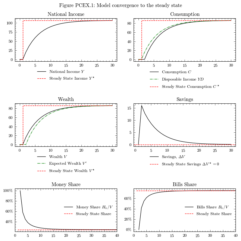
Convergence to the Steady State#
The steady state for Model PCEX is equivalent to model PC, it just has delays in reathing the steady state. In Godley and Lavoie [2006] models are initialized with almost all of the variables set to zero. For model PCEX the only non-zero item is that in period 0 the government demand is 20, i.e. the government creates 20 monetary units of demand.
To aid in our graphing, we can calculate the steady state solutions for the variables following the derivations in Section 4.5 of Godley and Lavoie Godley and Lavoie [2006]:
In macrostat, this solution has been implemented in the compute_theoretical_steady_state() function. We compute this now for scenario=0, which is the case without any shocks and constant government demand \(G\) and interest rates \(r\).
model.compute_theoretical_steady_state(scenario=0)
steadystate = model.variables.to_pandas()
INFO:root:Computing theoretical steady state. Scenario: 0
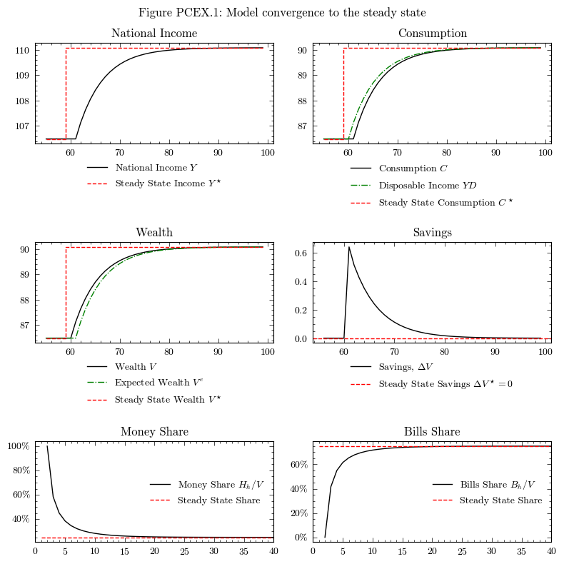
Perturbation 1: An increase of 100 points in the rate of interest on bills (\(r\))#
Following the convergence to the steady state, we can study the effects of an increase in the rate on bills by 100bps (Figures 4.3 and 4.4 in Godley and Lavoie [2006]).
MacroStat is set up to easily handle these scenarios. Much like in prior models, we simply define a new scenario IncreaseInterestRate and set the new rate to be 100 points higher \(r=0.025+0.01\)
model.parameters["scenario_trigger"] = 60
model.scenarios.add_scenario(
    name="IncreaseInterestRate",
    timeseries={"InterestRate":0.025 + 0.01}
)
model.simulate(scenario="IncreaseInterestRate")
output_rate_increase = model.variables.to_pandas()
INFO:root:Starting simulation. Scenario: 1
We then need to compute the new steady state values for the variables
model.compute_theoretical_steady_state(scenario="IncreaseInterestRate")
steadystate_rate_increase = model.variables.to_pandas()
INFO:root:Computing theoretical steady state. Scenario: 1
Now we can see how the model reacts to the shock.
Perturbation 2: An increase in the propensity to consume out of income (\(\alpha_1\))#
Following the convergence to the steady state, we can study the effects of an increase of the household sector’s propensity to consume out of income.
MacroStat is set up to easily handle time-dependent changes in the values of parameters (useful for scenarios and calibration). It specifically supports two types of paramer-shocks: multiplicative and additive. Thus, if pname is the name of the parameter, it checks for the existence of pname_multiply and pname_add in the scenarios to edit them.
Therefore, let us add this kind of scenario can easily be implemented in the MacroStat version by adding a scenario:
In the file
Scenariosspecific toGL06PCEX(i.e.macrostat/models/GL06PCEX/scenarios.py) I added thePropensityToConsumeIncome_adddefault_value, and set it to zero.Noting that we have convergence to the steady state at period 60, let us set this as the scenario trigger
We then need a new timeseries for the scenario, where we have
PropensityToConsumeIncome_add=0.01
model.parameters["scenario_trigger"] = 60
model.scenarios.add_scenario(
    name="PropensityToConsumeIncomeIncrease",
    timeseries={"PropensityToConsumeIncome_add":0.01}
)
model.simulate(scenario="PropensityToConsumeIncomeIncrease")
output_cons_propensity_increase = model.variables.to_pandas()
INFO:root:Starting simulation. Scenario: 2
We then need to compute the new steady state values for the variables
model.compute_theoretical_steady_state(scenario="PropensityToConsumeIncomeIncrease")
steadystate_cons_propensity_increase = model.variables.to_pandas()
INFO:root:Computing theoretical steady state. Scenario: 2
Now we can see how the model reacts to the shock.
