Model LP

Model LP is introduced in chapter 5 of Godley and Lavoie [2006] “Monetary Economics: An Integrated Approach to Credit, Money, Income, Production and Wealth”. It extends model PCEX by introducing long-term bonds, capital gains, and liquidity preference into the portfolio choice framework. Households now allocate their wealth across three assets: cash, Treasury bills, and long-term bonds.

Module Contents

As with all MacroStat models, LP is divided into Variables, Parameters (fixed constants), Scenarios, and the Behavior (model initialization and steps). The module-level documentation can be seen in:

• Variables
• Parameters
  • Hyperparameters
  • Parameters
• Equations
  • Initialization Equations
  • Step Equations
• Scenarios
  • Baseline
  • Scenario 1: Rise in Interest Rates (Section 5.7)
  • Scenario 2: Drop in alpha1 (Section 5.9)

The remainder of this page gives an introduction to the model, notes on how it is implemented in MacroStat and then shows some of the model dynamics by replicating the relevant graphs of Godley and Lavoie (2006).

Model Overview

Behavioral Equations

Model LP extends model PCEX by adding long-term bonds to the household portfolio. The key innovations are:

• Long-term bonds (\(BL\)) that pay a fixed coupon of 1 monetary unit per period

• Bond prices (\(p_{bl}\)) that are set exogenously and can generate capital gains (\(CG\))

• Three-asset portfolio choice across cash, bills, and bonds using Tobin’s framework

• Expected returns on bonds that combine yield and expected capital gains

1. National Income

(1)\[Y(t) = C(t) + G(t)\]

2. Disposable income now includes bond coupon income

(2)\[YD_r(t) = Y(t) - T(t) + r_b(t-1) \cdot B_h(t-1) + BL_h(t-1)\]

3. Taxes now include bond income in the tax base

(3)\[T(t) = \theta \cdot \left(Y(t) + r_b(t-1) \cdot B_h(t-1) + BL_h(t-1)\right)\]

4. Wealth now includes capital gains from bond price changes

(4)\[V(t) = V(t-1) + (YD_r(t) - C(t)) + CG(t)\]

5. Capital gains arise from bond price changes

(5)\[CG(t) = (p_{bl}(t) - p_{bl}(t-1)) \cdot BL_h(t-1)\]

6. Consumption (unchanged from PCEX)

(6)\[C(t) = \alpha_1 \cdot YD_r^e(t) + \alpha_2 \cdot V(t-1)\]

7. Expected wealth now includes capital gains

(7)\[V^e(t) = V(t-1) + (YD_r^e(t) - C(t)) + CG(t)\]

8. Bond yield is the inverse of the bond price

(8)\[r_{bl}(t) = \frac{1}{p_{bl}(t)}\]

9. Expected return on bonds combines yield and expected capital gain

(9)\[ERr_{bl}(t) = r_{bl}(t) + \chi \cdot \frac{p_{bl}^e(t) - p_{bl}(t)}{p_{bl}(t)}\]

10. In the base LP model, the expected bond price equals the current bond price (static expectations)

(10)\[p_{bl}^e(t) = p_{bl}(t)\]

11. Household demand for Treasury bills (Tobin portfolio allocation)

(11)\[B_d(t) = V^e(t) \cdot \lambda_{20} + V^e(t) \cdot (\lambda_{22} \cdot r_b(t) + \lambda_{23} \cdot ERr_{bl}(t)) + \lambda_{24} \cdot YD_r^e(t)\]

12. Household demand for bonds

(12)\[BL_d(t) = \frac{V^e(t) \cdot \left(\lambda_{30} + \lambda_{32} \cdot r_b(t) + \lambda_{33} \cdot ERr_{bl}(t) + \lambda_{34} \cdot \frac{YD_r^e(t)}{V^e(t)}\right)}{p_{bl}(t)}\]

13. Cash demand is the portfolio residual

(13)\[H_d(t) = V^e(t) - B_d(t) - p_{bl}(t) \cdot BL_d(t)\]

14. Portfolio holdings equal demands

(14)\[B_h(t) = B_d(t) \qquad BL_h(t) = BL_d(t)\]

15. Realized household cash holdings

(15)\[H_h(t) = V(t) - B_h(t) - p_{bl}(t) \cdot BL_h(t)\]

16. Government budget constraint now includes bond issuance

\begin{align} B_s(t) &= B_s(t-1) + G(t) + r_b(t-1) \cdot B_s(t-1) + BL_s(t-1) \\ &\quad - T(t) - r_b(t-1) \cdot B_{CB}(t-1) - (BL_s(t) - BL_s(t-1)) \cdot p_{bl}(t) \end{align}

17. Central bank bill holdings and money supply

\begin{align} B_{CB}(t) &= B_s(t) - B_h(t) \\ H_s(t) &= H_s(t-1) + (B_{CB}(t) - B_{CB}(t-1)) \end{align}

18. Expected disposable income (adaptive expectations)

(18)\[YD_r^e(t) = YD_r(t-1)\]

With the redundant equation being

(19)\[H_s(t) = H_h(t)\]

Note

In Model LP, the expected bond price \(p_{bl}^e = p_{bl}\) (static expectations), so the expected capital gain term in \(ERr_{bl}\) is always zero, and \(ERr_{bl} = r_{bl} = 1/p_{bl}\). Models LP2 and LP3 introduce adaptive expectations where \(p_{bl}^e \neq p_{bl}\).

Transaction Flow Matrix

Accounting Transaction Matrix for Model LP

	Household	Production	Government	CentralBank	CentralBank	Total
	Current	Current	Current	Current	Capital
Consumption Household	\(-C(t)\)	\(+C(t)\)				\(0\)
Consumption Government		\(+G(t)\)	\(-G(t)\)			\(0\)
National Income	\(+Y(t)\)	\(-Y(t)\)				\(0\)
Taxes	\(-T(t)\)		\(+T(t)\)			\(0\)
Interest On Bills Household	\(+r_b(t-1) \cdot B_h(t-1)\)		\(-r_b(t-1) \cdot B_h(t-1)\)			\(0\)
Bond Coupon Income Household	\(+BL_h(t-1)\)		\(-BL_h(t-1)\)			\(0\)
Central Bank Profits			\(+r_b(t-1) \cdot B_{CB}(t-1)\)	\(-r_b(t-1) \cdot B_{CB}(t-1)\)		\(0\)
Change in Bill Stock	\(+\Delta B_h(t)\)		\(-\Delta B_s(t)\)		\(+\Delta B_{CB}(t)\)	\(0\)
Change in Bond Stock	\(+\Delta BL_h(t)\)					\(0\)
Change in Bond Supply			\(-\Delta BL_s(t)\)			\(0\)
Change in Cash Stock	\(+\Delta H_h(t)\)					\(0\)
Change in Money Stock					\(-\Delta H_s(t)\)	\(0\)
Total	\(0\)	\(0\)	\(0\)	\(0\)	\(0\)	\(0\)

Balance Sheet Matrix

Balance Sheet for Model LP

	Household	Production	Government	CentralBank	Total
	Current	Current	Current	Capital
Wealth	\(-V(t)\)		\(+V(t)\)		0
Bill Stock	\(+B_h(t)\)		\(-B_s(t)\)	\(+B_{CB}(t)\)	0
Bond Stock	\(+BL_h(t)\)				0
Bond Supply			\(-BL_s(t)\)		0
Cash Stock	\(+H_h(t)\)				0
Money Stock				\(-H_s(t)\)	0

Implementation in MacroStat

Transposing these equations to the MacroStat framework, we consider that there are:

1. Twelve parameters (fixed constants): \(\alpha_1\), \(\alpha_2\), \(\theta\), \(\chi\), and the eight \(\lambda\) portfolio coefficients (see Parameters)

2. Three scenario variables: \(G(t)\), \(r_b(t)\), and \(p_{bl}(t)\) (see Scenarios)

3. The remaining tracked series are variables (see Variables)

Model Dynamics

Preparatory Steps

%load_ext autoreload
%autoreload 2

import importlib
import logging
import sys

# Import the necessary libraries for plotting
from matplotlib import pyplot as plt
from matplotlib.ticker import PercentFormatter

# Import the MacroStat model components
from macrostat.models.GL06LP import GL06LP, ParametersGL06LP, ScenariosGL06LP

# Custom matplotlib style for the documentation
plt.style.use("../../macrostat.mplstyle")
# We show the logging output in the notebook
importlib.reload(logging)
logging.basicConfig(stream=sys.stdout, level=logging.INFO)

Running the Simulation

First, we can run the model without any shocks to see the convergence to the steady state.

params = ParametersGL06LP()
model = GL06LP(parameters=params)
model.simulate()
output = model.variables.to_pandas()

We can check that the variables are healthy, meaning the redundant equation \(H_h = H_s\) holds and all stocks are positive.

Note

Due to floating point precision, the redundant equation will not hold exactly. We check that the absolute percentage error is below a tolerance.

model.variables.check_health(tolerance=1e-3)

True

An overview of the first 10 steps of the model:

df = model.variables.to_pandas()
df.head(10).T

	time	0	1	2	3	4	5	6	7	8	9
ConsumptionHousehold	Household	0.0	0.0	0.000000	16.124001	29.123171	40.013660	49.124569	56.747089	63.124352	68.459801
ConsumptionGovernment	Government	0.0	0.0	20.000000	20.000000	20.000000	20.000000	20.000000	20.000000	20.000000	20.000000
NationalIncome	Macroeconomy	0.0	0.0	20.000000	36.124001	49.123169	60.013660	69.124573	76.747086	83.124352	88.459801
Taxes	Household	0.0	0.0	3.876000	7.000832	9.618765	11.808908	13.641264	15.174274	16.456844	17.529890
InterestOnBillsHousehold	Household	0.0	0.0	0.000000	0.000000	0.191050	0.345075	0.474114	0.582067	0.672385	0.747948
BondCouponIncomeHousehold	Household	0.0	0.0	0.000000	0.000000	0.318207	0.574746	0.789669	0.969473	1.119904	1.245759
CentralBankProfits	CentralBank	0.0	0.0	0.000000	0.483720	0.491721	0.510488	0.525822	0.538661	0.549403	0.558390
CapitalGains	Household	0.0	0.0	0.000000	0.000000	0.000000	0.000000	0.000000	0.000000	0.000000	0.000000
ExpectedCapitalGains	Household	0.0	0.0	0.000000	0.000000	0.000000	0.000000	0.000000	0.000000	0.000000	0.000000
Wealth	Household	0.0	0.0	16.124001	29.123169	40.013657	49.124569	56.747089	63.124355	68.459801	72.923622
HouseholdBillStock	Household	0.0	0.0	0.000000	6.368336	11.502485	15.803792	19.402239	22.412830	24.931595	27.038883
GovernmentBillStock	Government	0.0	0.0	16.124001	22.759026	28.518745	33.331181	37.357616	40.726269	43.544609	45.902531
CentralBankBillStock	CentralBank	0.0	0.0	16.124001	16.390690	17.016260	17.527390	17.955378	18.313438	18.613014	18.863647
HouseholdBondStock	Household	0.0	0.0	0.000000	0.318207	0.574746	0.789669	0.969473	1.119904	1.245759	1.351054
GovernmentBondSupply	Government	0.0	0.0	0.000000	0.318207	0.574746	0.789669	0.969473	1.119904	1.245759	1.351054
HouseholdCashStock	Household	0.0	0.0	16.124001	16.390690	17.016258	17.527390	17.955381	18.313450	18.613026	18.863657
CentralBankMoneyStock	CentralBank	0.0	0.0	16.124001	16.390690	17.016262	17.527391	17.955379	18.313440	18.613014	18.863647
DisposableIncome	Household	0.0	0.0	16.124001	29.123169	40.013660	49.124569	56.747089	63.124352	68.459801	72.923615
ExpectedDisposableIncome	Household	0.0	0.0	0.000000	16.124001	29.123169	40.013660	49.124569	56.747089	63.124352	68.459801
ExpectedWealth	Household	0.0	0.0	0.000000	16.124001	29.123167	40.013653	49.124569	56.747089	63.124352	68.459801
HouseholdBillDemand	Household	0.0	0.0	0.000000	6.368336	11.502485	15.803792	19.402239	22.412830	24.931595	27.038883
HouseholdBondDemand	Household	0.0	0.0	0.000000	0.318207	0.574746	0.789669	0.969473	1.119904	1.245759	1.351054
HouseholdCashDemand	Household	0.0	0.0	0.000000	3.391522	6.125768	8.416473	10.332863	11.936184	13.277576	14.399836
InterestRateBills	Macroeconomy	0.0	0.0	0.030000	0.030000	0.030000	0.030000	0.030000	0.030000	0.030000	0.030000
BondPrice	Macroeconomy	0.0	0.0	20.000000	20.000000	20.000000	20.000000	20.000000	20.000000	20.000000	20.000000
BondYield	Macroeconomy	0.0	0.0	0.050000	0.050000	0.050000	0.050000	0.050000	0.050000	0.050000	0.050000
ExpectedBondPrice	Household	0.0	0.0	20.000000	20.000000	20.000000	20.000000	20.000000	20.000000	20.000000	20.000000
ExpectedReturnOnBonds	Household	0.0	0.0	0.050000	0.050000	0.050000	0.050000	0.050000	0.050000	0.050000	0.050000

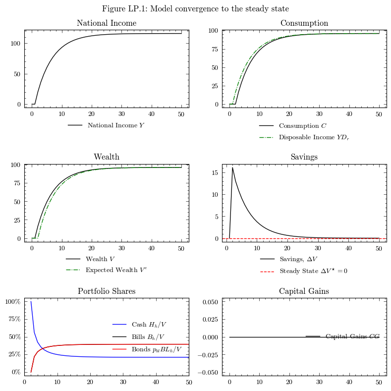
Convergence to the Steady State

In the steady state of Model LP (with constant bond prices), capital gains are zero, and the model behaves similarly to PCEX but with three-asset portfolio choice. The household allocates its wealth across cash, Treasury bills, and bonds according to the Tobin portfolio equations.

Unlike earlier models, an analytical closed-form steady state is not straightforward for Model LP due to the additional portfolio equations and the interaction between bond yields and portfolio allocation. We therefore rely on the numerical convergence of the simulation.

dfo = output.loc[:50]

fig, axs = plt.subplots(ncols=2, nrows=3, figsize=(8, 8))

# National Income
axs[0, 0].plot(dfo.index, dfo['NationalIncome'], color='k', label=r'National Income $Y$')
axs[0, 0].legend(loc='upper center', bbox_to_anchor=(0.5, -0.1), frameon=False)
axs[0, 0].set_title('National Income')

# Consumption and Disposable Income
axs[0, 1].plot(dfo.index, dfo['ConsumptionHousehold'], color='k', label=r'Consumption $C$')
axs[0, 1].plot(dfo.index, dfo['DisposableIncome'], color='g', linestyle='-.', label=r'Disposable Income $YD_r$')
axs[0, 1].legend(loc='upper center', bbox_to_anchor=(0.5, -0.1), frameon=False)
axs[0, 1].set_title('Consumption')

# Wealth
axs[1, 0].plot(dfo.index, dfo['Wealth'], color='k', label=r'Wealth $V$')
axs[1, 0].plot(dfo.index, dfo['ExpectedWealth'], color='g', linestyle='-.', label=r'Expected Wealth $V^e$')
axs[1, 0].legend(loc='upper center', bbox_to_anchor=(0.5, -0.1), frameon=False)
axs[1, 0].set_title('Wealth')

# Savings
axs[1, 1].plot(dfo.index, dfo['Wealth'].diff(), color='k', label=r'Savings, $\Delta V$')
axs[1, 1].axhline(y=0, color='r', linestyle='--', label=r'Steady State $\Delta V^\star=0$')
axs[1, 1].legend(loc='upper center', bbox_to_anchor=(0.5, -0.1), frameon=False)
axs[1, 1].set_title('Savings')

# Portfolio Shares
cash_share = output['HouseholdCashStock'] / output['Wealth']
bill_share = output['HouseholdBillStock'] / output['Wealth']
bond_share = (output['HouseholdBondStock'].mul(output[('BondPrice','Macroeconomy')],axis=0)) / output['Wealth']

axs[2, 0].plot(output.index, cash_share, color='b', label='Cash $H_h/V$')
axs[2, 0].plot(output.index, bill_share, color='k', label='Bills $B_h/V$')
axs[2, 0].plot(output.index, bond_share, color='r', label='Bonds $p_{bl} BL_h/V$')
axs[2, 0].legend(loc='center right', frameon=False)
axs[2, 0].set_xlim(0, 50)
axs[2, 0].set_title('Portfolio Shares')
axs[2, 0].yaxis.set_major_formatter(PercentFormatter(1))

# Capital Gains
axs[2, 1].plot(dfo.index, dfo['CapitalGains'], color='k', label=r'Capital Gains $CG$')
axs[2, 1].set_title('Capital Gains')
axs[2, 1].legend(loc='center right', frameon=False)

fig.suptitle('Figure LP.1: Model convergence to the steady state')
plt.tight_layout()
plt.show()

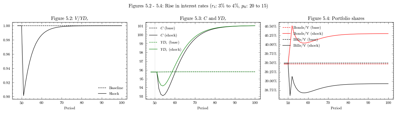
Perturbation 1: Increase in both short-term and long-term interest rates (Section 5.7)

Following Section 5.7 of Godley and Lavoie [2006], we suppose there is an unexpected increase in the interest rates set by the monetary authorities. The bill rate rises from 3% to 4%, while the bond price drops from 20 to 15 (the bond yield rises from 5% to 6.67%). With static expectations (\(p_{bl}^e = p_{bl}\)), the expected return on bonds rises by the same amount as the yield.

The most important point of this experiment is that the fall in bond prices induces an immediate reduction in wealth through capital losses. This is one of the main conduits for monetary policy — a rise in interest rates reduces demand temporarily through the wealth channel in the consumption function. However, in the long run, the effect of higher interest rates is positive because higher debt service payments increase household income.

scenarios = ScenariosGL06LP(parameters=params)
sc1 = scenarios.get_scenario_index("Scenario.1: Rise in interest rates")
model1 = GL06LP(parameters=params, scenarios=scenarios)
model1.simulate(scenario=sc1)
output_sc1 = model1.variables.to_pandas()

trigger = params["scenario_trigger"]
dfo = output_sc1.loc[trigger - 2:]
dfo_base = output.loc[trigger - 2:]

fig, axes = plt.subplots(1, 3, figsize=(14, 4))

# Figure 5.2: V/YDr ratio
v_yd_base = dfo_base['Wealth'] / dfo_base['DisposableIncome']
v_yd_shock = dfo['Wealth'] / dfo['DisposableIncome']
axes[0].plot(dfo_base.index, v_yd_base, 'k--', label='Baseline')
axes[0].plot(dfo.index, v_yd_shock, 'k-', label='Shock')
axes[0].axvline(x=trigger, color='grey', linestyle=':', alpha=0.5)
axes[0].set_title('Figure 5.2: $V / YD_r$')
axes[0].set_xlabel('Period')
axes[0].legend(frameon=False)

# Figure 5.3: C and YDr
axes[1].plot(dfo_base.index, dfo_base['ConsumptionHousehold'], 'k--', label='$C$ (base)')
axes[1].plot(dfo.index, dfo['ConsumptionHousehold'], 'k-', label='$C$ (shock)')
axes[1].plot(dfo_base.index, dfo_base['DisposableIncome'], 'g--', label='$YD_r$ (base)')
axes[1].plot(dfo.index, dfo['DisposableIncome'], 'g-', label='$YD_r$ (shock)')
axes[1].axvline(x=trigger, color='grey', linestyle=':', alpha=0.5)
axes[1].set_title('Figure 5.3: $C$ and $YD_r$')
axes[1].set_xlabel('Period')
axes[1].legend(frameon=False)

# Figure 5.4: portfolio shares
bond_share_sc1 = output_sc1['HouseholdBondStock'].mul(output_sc1[('BondPrice',"Macroeconomy")],axis=0).div(output_sc1['Wealth'])
bill_share_sc1 = output_sc1['HouseholdBillStock'] / output_sc1['Wealth']
bond_share_base = output['HouseholdBondStock'].mul(output[('BondPrice',"Macroeconomy")],axis=0).div(output['Wealth'])
bill_share_base = output['HouseholdBillStock'] / output['Wealth']

axes[2].plot(bond_share_base.loc[trigger - 2:].index, bond_share_base.loc[trigger - 2:], 'r--', label='Bonds/V (base)')
axes[2].plot(bond_share_sc1.loc[trigger - 2:].index, bond_share_sc1.loc[trigger - 2:], 'r-', label='Bonds/V (shock)')
axes[2].plot(bill_share_base.loc[trigger - 2:].index, bill_share_base.loc[trigger - 2:], 'k--', label='Bills/V (base)')
axes[2].plot(bill_share_sc1.loc[trigger - 2:].index, bill_share_sc1.loc[trigger - 2:], 'k-', label='Bills/V (shock)')
axes[2].axvline(x=trigger, color='grey', linestyle=':', alpha=0.5)
axes[2].set_title('Figure 5.4: Portfolio shares')
axes[2].set_xlabel('Period')
axes[2].yaxis.set_major_formatter(PercentFormatter(1))
axes[2].legend(frameon=False)

fig.suptitle('Figures 5.2 - 5.4: Rise in interest rates ($r_b$: 3% to 4%, $p_{bl}$: 20 to 15)')
plt.tight_layout()
plt.show()

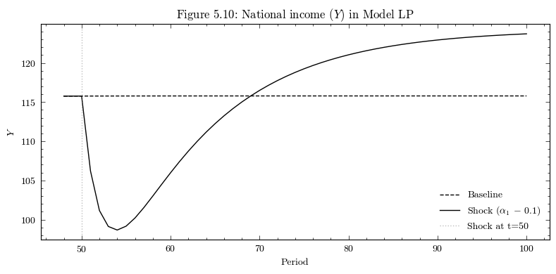
Perturbation 2: Sharp decrease in propensity to consume (Section 5.9, LP baseline)

Following Section 5.9 of Godley and Lavoie [2006], we reduce the propensity to consume out of current income (\(\alpha_1\)) by 0.1. This has a negative short-run impact on GDP, but in Model LP (with exogenous government spending), the economy eventually recovers above the initial steady state. The larger saving leads to more government debt, higher interest payments, and hence higher disposable income in the long run.

This result serves as the crucial comparison with Model LP3 (Figure 5.10 vs Figure 5.11), where the fiscal austerity rule prevents the recovery.

scenarios = ScenariosGL06LP(parameters=params)
sc2 = scenarios.get_scenario_index("Scenario.2: Drop in alpha1")
model2 = GL06LP(parameters=params, scenarios=scenarios)
model2.simulate(scenario=sc2)
output_sc2 = model2.variables.to_pandas()

dfo = output_sc2.loc[trigger - 2:]

fig, ax = plt.subplots(figsize=(8, 4))
ax.plot(dfo_base.index, dfo_base['NationalIncome'], 'k--', label='Baseline')
ax.plot(dfo.index, dfo['NationalIncome'], 'k-', label='Shock ($\\alpha_1$ − 0.1)')
ax.axvline(x=trigger, color='grey', linestyle=':', alpha=0.5, label=f'Shock at t={trigger}')
ax.set_title('Figure 5.10: National income ($Y$) in Model LP')
ax.set_xlabel('Period')
ax.set_ylabel('$Y$')
ax.legend(frameon=False)
plt.tight_layout()
plt.show()