New Keynesian 3-Equation (NK3E)

import os
import sys
import math
import numpy as np
import pandas as pd

# Optional plotting
try:
    import matplotlib.pyplot as plt
    HAVE_PLT = True
except Exception:
    HAVE_PLT = False

# Ensure src is on path if running notebook directly
root = os.path.abspath(os.path.join(os.getcwd()))
src_path = os.path.join(root, "src")
if os.path.isdir(src_path) and src_path not in sys.path:
    sys.path.insert(0, src_path)

from macrostat.models.NK3E import (
    NK3E,
    ParametersNK3E,
    VariablesNK3E,
    ScenariosNK3E,
)

# Configure a short horizon and ensure no tqdm
params = ParametersNK3E(
    hyperparameters={
        "timesteps": 50,
        "timesteps_initialization": 1,
        "use_tqdm": False,
    }
)
variables = VariablesNK3E(parameters=params)
scenarios = ScenariosNK3E(parameters=params)
model = NK3E(parameters=params, variables=variables, scenarios=scenarios)

print("Model ready: NK3E with", params["timesteps"], "timesteps")

Model ready: NK3E with 50 timesteps

# Baseline simulation
model.simulate()
ts = model.variables.timeseries

# Tensor to numpy helper
_to_np = lambda x: x.detach().cpu().squeeze().numpy() if hasattr(x, "detach") else np.asarray(x)

# Collect into a DataFrame for convenience
baseline_df = pd.DataFrame({
    "y": _to_np(ts["y"]),
    "pi": _to_np(ts["pi"]),
    "r": _to_np(ts["r"]),
    "r_s": _to_np(ts["r_s"]),
})

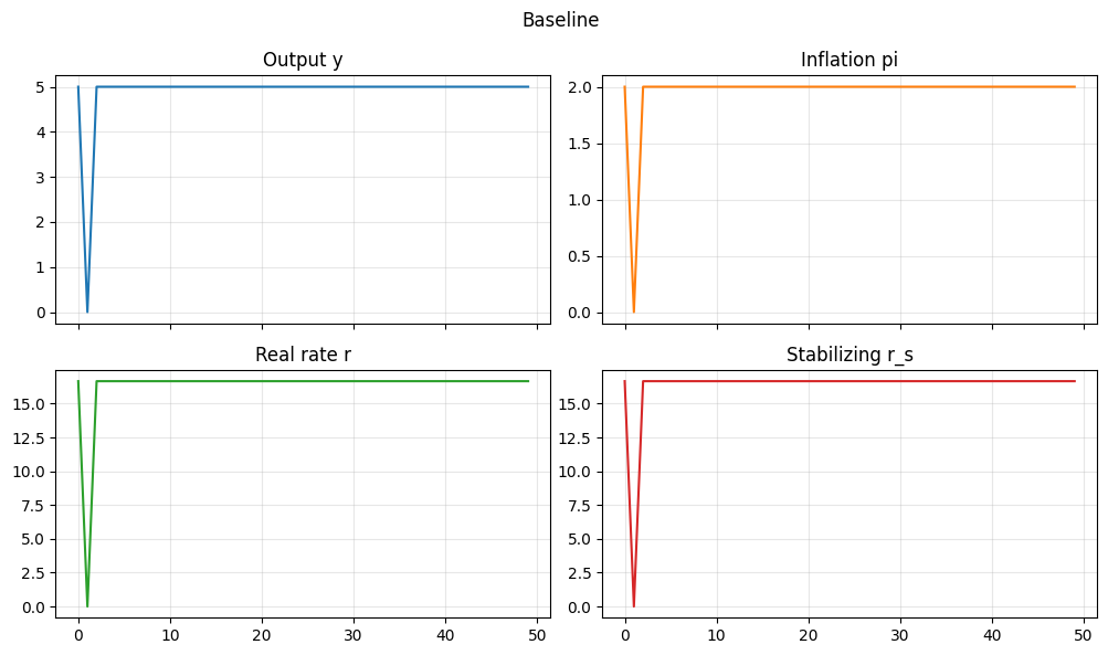
baseline_df.tail()

	y	pi	r	r_s
45	5.0	2.0	16.666666	16.666666
46	5.0	2.0	16.666666	16.666666
47	5.0	2.0	16.666666	16.666666
48	5.0	2.0	16.666666	16.666666
49	5.0	2.0	16.666666	16.666666

# Scenario runs
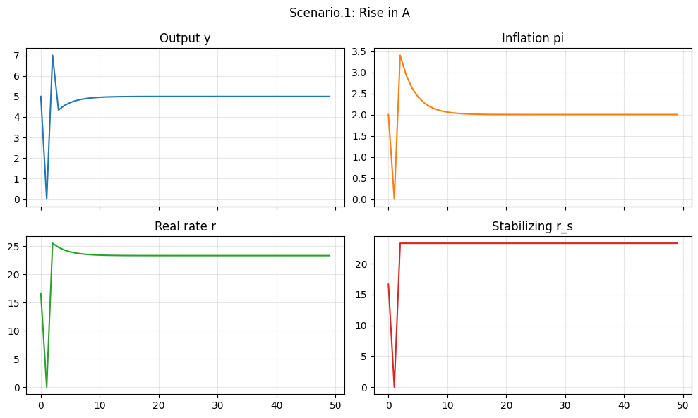
scenario_names = [
    "Scenario.1: Rise in A",
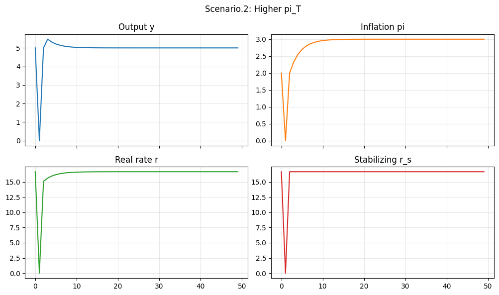
    "Scenario.2: Higher pi_T",
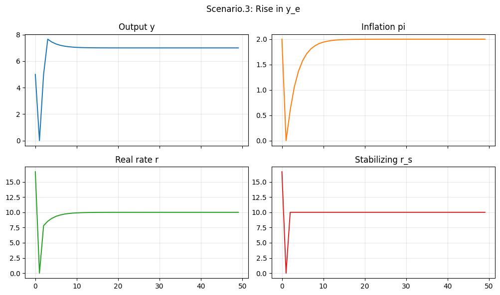
    "Scenario.3: Rise in y_e",
]

scenario_dfs = {}
for name in scenario_names:
    model.simulate(scenario=name)
    ts = model.variables.timeseries
    scenario_dfs[name] = pd.DataFrame({
        "y": _to_np(ts["y"]),
        "pi": _to_np(ts["pi"]),
        "r": _to_np(ts["r"]),
        "r_s": _to_np(ts["r_s"]),
    })

{ k: v.tail(1) for k, v in scenario_dfs.items() }

{'Scenario.1: Rise in A':       y   pi          r        r_s
 49  5.0  2.0  23.333332  23.333332,
 'Scenario.2: Higher pi_T':       y   pi          r        r_s
 49  5.0  3.0  16.666666  16.666666,
 'Scenario.3: Rise in y_e':       y        pi         r   r_s
 49  7.0  1.999999  9.999999  10.0}

def plot_series(df, title):
    if not HAVE_PLT:
        print(f"Skipping plots for '{title}' (matplotlib not available)")
        return
    fig, axs = plt.subplots(2, 2, figsize=(10, 6), sharex=True)
    axs = axs.ravel()
    axs[0].plot(df["y"], label="y"); axs[0].set_title("Output y")
    axs[1].plot(df["pi"], label="pi", color="tab:orange"); axs[1].set_title("Inflation pi")
    axs[2].plot(df["r"], label="r", color="tab:green"); axs[2].set_title("Real rate r")
    axs[3].plot(df["r_s"], label="r_s", color="tab:red"); axs[3].set_title("Stabilizing r_s")
    for ax in axs:
        ax.grid(True, alpha=0.3)
    fig.suptitle(title)
    plt.tight_layout()
    plt.show()

plot_series(baseline_df, "Baseline")
for name, df in scenario_dfs.items():
    plot_series(df, name)