Model SIM

Model SIM is introduced in chapter 3 of Godley and Lavoie [2006] “Monetary Economics: An Integrated Approach to Credit, Money, Income, Production and Wealth” and represents the “simplest model with government money”. That is, this is a model with only outside money (from the government).

Module Contents

As with all MacroStat models, SIM is divided into Variables, Parameters (fixed constants), Scenarios, and the Behavior (model initialization and steps). The module-level documentation, such as all variables/parameters/scenarios and their notation or the behavioral equations associated with each function of BehaviorSIM.py can be seen in:

• Variables
• Parameters
  • Hyperparameters
  • Parameters
• Equations
  • Initialization
  • Main Simulation Loop
• Scenarios

Note

The remainder of this page gives an introduction to the model, notes on how it is implemented in MacroStat and then shows some of the model dynamics by replicating the relevant graphs of Godley and Lavoie (2006).

Model Overview

Behavioral Equations

The SIM model is introduced in Chapter 3, and consists of the following 11 equations and 11 unknowns:

1. Consumption good supply equals demand

(1)\[C_s(t) = C_d(t)\]

2. Governmend good supply equals demand

(2)\[G_s(t) = G_d(t)\]

3. Tax supply equals demand

(3)\[T_s(t) = T_d(t)\]

4. Labour supply equals demand

(4)\[N_s(t) = N_d(t)\]

5. Disposable income is wage income minus taxes

(5)\[YD(t) = W(t)\cdot N_s(t) - T_s(t)\]

6. Tax demand is a fixed proportion of wage income

(6)\[T_d(t) = \theta\cdot W(t)\cdot N_s(t)\]

7. Consumption demand is a share of disposable income and deposits

(7)\[C_d(t) = \alpha_1\cdot YD(t) + \alpha_2\cdot H_h(t-1)\]

8. The change in government stock of money is demand minus tax

(8)\[\Delta H_s(t) = H_s(t) - H_s(t-1) = G_d(t) - T_d(t)\]

9. The change in household deposits is disposable income minus expenditure

(9)\[\Delta H_h(t) = H_h(t) - H_h(t-1) = YD(t) - C_d(t)\]

8. Total national income is consumption of households and government

(10)\[Y(t) = C_s(t) + G_s(t)\]

8. Labour Demand is national income over wages

(11)\[N_d(t) = \frac{Y(t)}{W(t)}\]

With the redundant equation being

(12)\[\Delta H_s(t) = \Delta H_h(t)\]

Transaction Flow Matrix

The accounting of transactions for model SIM is as follows:

Accounting Transaction Matrix for Model SIM

	Household	Production	Government	Total
	Current	Current	Current
Consumption Supply	\(-C_s(t)\)	\(+C_s(t)\)		\(0\)
Government Supply		\(+G_s(t)\)	\(-G_s(t)\)	\(0\)
Tax Supply	\(-T_s(t)\)		\(+T_s(t)\)	\(0\)
Labour Earnings	\(+W(t)\cdot N_s(t)\)	\(-W(t)\cdot N_s(t)\)		\(0\)
Change in Money Stock	\(+H_h(t)\)		\(-H_s(t)\)	\(0\)
Total	\(0\)	\(0\)	\(0\)	\(0\)

Balance Sheet Matrix

Balance Sheet for Model SIM

	Household	Production	Government	Total
	Current	Current	Current
Money Stock	\(+H_h(t)\)		\(-H_s(t)\)	0

Implementation in MacroStat

Transposing these eleven equations to the MacroStat framework, we consider that there are:

1. Three parameters (fixed constants): \(\alpha_1\), \(\alpha_2\), and \(\theta\) (see Parameters)

2. Two scenario variables : \(G_d(t)\) and \(W(t)\) (see Scenarios)

3. The remaining 14 tracked series are variables (see Variables)

Behavioral Modeling

For the implementation of the behavioral equations (see Behavior), most prior implementations have made use of some form of linear solver or iteration until the system is solved. To simplify the implementation in Macrostat, we can note that the system can be solved analytically for a given timestep as follows:

Substitute into Eq. (11) to obtain

\[N_d(t) =\frac{1}{W(t)}(C_d(t) + G_d(t))\]

where we can already note that \(W(t)\) and \(G_d(t)\) are exogenously given (they are scenario variables). This leaves us to solve for \(C_d(t)\), where we can use Eq. (7) and Eq. (5) to obtain

\[N_d(t) =\frac{1}{W(t)}(\alpha_1(1-\theta)W(t)N_s(t) + \alpha_2 H_h(t-1) + G_d)\]

now noting from Eq. (4) that supply=demand, we can rewrite the above as

(13)\[N_d(t) =\frac{\alpha_2 H_h(t-1) + G_d}{W(t)(1-\alpha_1(1-\theta))}\]

Therefore, for a given period \(t\) we can solve the system by solving, in order:

1. Eq. (2) given the scenario variable

2. Eq. (13) for labour demand based on prior information \(H_h(t)\) and scenario variables \(W(t)\) and \(G_d(t)\) (this replaces the need to run Eq. (11))

3. Eq. (4)

4. Tax demand, given labour, Eq. (6)

5. Tax supply, given demand, Eq. (3)

6. Disposable income, given labour supply and tax demand, Eq. (5)

7. Consumption demand, given disposable income, Eq. (7)

8. Consumption supply, given demand, Eq. (1)

9. Government stock of money, Eq. (8)

10. Household stock of deposits, Eq. (9)

11. National income, Eq. (10)

This is implemented as such in the Behavior class.

Model Dynamics

Preparatory Steps

%load_ext autoreload
%autoreload 2

from matplotlib import pyplot as plt
from macrostat.models import get_model
from macrostat.util import latex_model_description

plt.style.use("../../macrostat.mplstyle")

The autoreload extension is already loaded. To reload it, use:
  %reload_ext autoreload

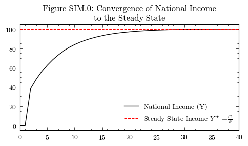
Convergence to the Steady State

In Godley and Lavoie [2006] models are initialized with almost all of the variables set to zero. For model SIM the only non-zero item is that in period 0 the government demand is 20, i.e. the government creates 20 monetary units of demand. Thereafter the system converges to a steady state. We can see this by simulating the default parameters and checking that total national income is 100.

GLO6SIM = get_model("GL06SIM")
model = GLO6SIM()
model.simulate()
output = model.variables.to_pandas()

latex_model_description.make_latex_model_description(GLO6SIM().behavior)

The consumption demand is a function of the disposable income, the propensity to consume income, and the propensity to consume savings. Equation (3.7) in the book.
In the model it is assumed that the supply will adjust to the demand, that is, whatever is demanded can and will be produced. Equation (3.1) in the book.
The disposable income is the wage bill minus the taxes. Equation (3.5) in the book.
The government money stock is a function of the government demand, and the tax supply. Equation (3.8) in the book.
In the model it is assumed that the supply will adjust to the demand, that is, whatever is demanded can and will be produced. Equation (3.2) in the book.
The household money stock is a function of the disposable income, the propensity to consume income, and the propensity to consume savings. Equation (3.9) in the book.
We can resolve the labour demand from the national income equation, together with the consumption demand (+ disposable income) and the government demand knowing that labour demand is equal to labour supply.
The labour income is the wage rate times the labour supply. This is an intermediate variable used to calculate the disposable income, but is computed explicitly here to compute the transaction flows.
In the model it is assumed that the supply will be equal to the amount of labour demanded. Equation (3.4) in the book
The national income is the sum of the consumption demand, the government demand, and the tax supply. Equation (3.10) in the book.
The tax demand is a function of the tax rate, the labour supply, and the wage rate. Equation (3.6) in the book.
In the model it is assumed that the supply will be equal to the amount of taxes demanded. Equation (3.3) in the book

'\\documentclass{article}\n\\usepackage{amsmath}\n\\usepackage{amssymb}\n\\begin{document}\n\\title{BehaviorGL06SIM}\n\\maketitle\n\\section{Step Equations}\n\\subsection{Consumption Demand}\nThe consumption demand is a function of the disposable income, the propensity to consume income, and the propensity to consume savings. Equation (3.7) in the book.\n\n\\begin{align}\\label{eq:consumption_demand}\nC_d(t) = \\alpha_1 YD(t) + \\alpha_2 H_h(t-1)\n\\end{align}\n\n\n\\subsection{Consumption Supply}\nIn the model it is assumed that the supply will adjust to the demand, that is, whatever is demanded can and will be produced. Equation (3.1) in the book.\n\n\\begin{align}\\label{eq:consumption_supply}\nC_s(t) = C_d(t)\n\\end{align}\n\n\n\\subsection{Disposable Income}\nThe disposable income is the wage bill minus the taxes. Equation (3.5) in the book.\n\n\\begin{align}\\label{eq:disposable_income}\nYD(t) = W(t) N_s(t) - T_s(t)\n\\end{align}\n\n\n\\subsection{Government Money Stock}\nThe government money stock is a function of the government demand, and the tax supply. Equation (3.8) in the book.\n\n\\begin{align}\\label{eq:government_money_stock}\nH_s(t) = H_s(t-1) + G_d(t) - T_d(t)\n\\end{align}\n\n\n\\subsection{Government Supply}\nIn the model it is assumed that the supply will adjust to the demand, that is, whatever is demanded can and will be produced. Equation (3.2) in the book.\n\n\\begin{align}\\label{eq:government_supply}\nG_s(t) = G_d(t)\n\\end{align}\n\n\n\\subsection{Household Money Stock}\nThe household money stock is a function of the disposable income, the propensity to consume income, and the propensity to consume savings. Equation (3.9) in the book.\n\n\\begin{align}\\label{eq:household_money_stock}\nH_h(t) = H_h(t-1) + YD(t) - C_d(t)\n\\end{align}\n\n\n\\subsection{Labour Demand}\nWe can resolve the labour demand from the national income equation, together with the consumption demand (+ disposable income) and the government demand knowing that labour demand is equal to labour supply.\n\n\\begin{align}\\label{eq:labour_demand}\nN_d(t) =\\frac{\\alpha_2 H_h(t-1) + G_d}{W(t)(1-\\alpha_1(1-\\theta))}\n\\end{align}\n\n\n\\subsection{Labour Income}\nThe labour income is the wage rate times the labour supply. This is an intermediate variable used to calculate the disposable income, but is computed explicitly here to compute the transaction flows.\n\n\\begin{align}\\label{eq:labour_income}\nW(t) N_s(t)\n\\end{align}\n\n\n\\subsection{Labour Supply}\nIn the model it is assumed that the supply will be equal to the amount of labour demanded. Equation (3.4) in the book\n\n\\begin{align}\\label{eq:labour_supply}\nN_s(t) = N_d(t)\n\\end{align}\n\n\n\\subsection{National Income}\nThe national income is the sum of the consumption demand, the government demand, and the tax supply. Equation (3.10) in the book.\n\n\\begin{align}\\label{eq:national_income}\nY(t) = C_s(t) + G_s(t)\n\\end{align}\n\n\n\\subsection{Tax Demand}\nThe tax demand is a function of the tax rate, the labour supply, and the wage rate. Equation (3.6) in the book.\n\n\\begin{align}\\label{eq:tax_demand}\nT_d(t) = \\theta N_s(t) W(t)\n\\end{align}\n\n\n\\subsection{Tax Supply}\nIn the model it is assumed that the supply will be equal to the amount of taxes demanded. Equation (3.3) in the book\n\n\\begin{align}\\label{eq:tax_supply}\nT_s(t) = T_d(t)\n\\end{align}\n\n\n\\end{document}'

National Income

steady_state_income = model.scenarios[(0,"GovernmentDemand")][0] / model.parameters["TaxRate"]

fig, axs = plt.subplots(1, 1, figsize=(5, 3))
axs.plot(output.index, output['NationalIncome'], color='k', label='National Income (Y)')
axs.axhline(y=steady_state_income, color='r', linestyle='--', label=r'Steady State Income $Y^\star=\frac{G}{\theta}$')
axs.legend(loc='lower right', frameon=False)
axs.set_xlim(0,40)
axs.set_title('Figure SIM.0: Convergence of National Income\nto the Steady State')
plt.tight_layout()
plt.show()

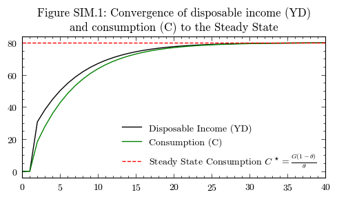
Disposable Income and Consumption

Corresponding to Figure 3.2 “Disposable income and consumption starting from scratch”

steady_state_consumption= (model.scenarios[(0,"GovernmentDemand")][0] * (1-model.parameters["TaxRate"])) / model.parameters["TaxRate"]

fig, axs = plt.subplots(1, 1, figsize=(5, 3))
axs.plot(output.index, output['DisposableIncome'], color='k', label='Disposable Income (YD)')
axs.plot(output.index, output['ConsumptionDemand'], color='g', label='Consumption (C)')
axs.axhline(y=steady_state_consumption, color='r', linestyle='--', label=r'Steady State Consumption $C^\star=\frac{G(1-\theta)}{\theta}$')
axs.legend(loc='lower right', frameon=False)
axs.set_xlim(0,40)
axs.set_title('Figure SIM.1: Convergence of disposable income (YD)\nand consumption (C) to the Steady State')
plt.tight_layout()
plt.show()

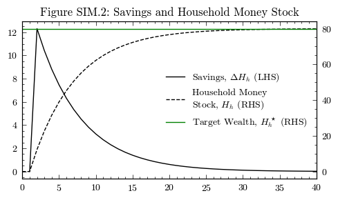
Wealth and Savings

Corresponding to Figure 3.3 “Wealth change and wealth level, starting from scratch (Table 3.4)”

alpha3 = (1-model.parameters["PropensityToConsumeSavings"]) / model.parameters["PropensityToConsumeIncome"]
steady_state_wealth = alpha3 * (model.scenarios[(0,"GovernmentDemand")][0] * (1-model.parameters["TaxRate"])) / model.parameters["TaxRate"]

fig, axs = plt.subplots(1, 1, figsize=(5, 3))
line1 = axs.plot(output.index, output['HouseholdMoneyStock'].diff(), color='k', label='Savings, $\Delta H_h$ (LHS)')
ax2 = axs.twinx()
line2 = ax2.plot(output.index, output['HouseholdMoneyStock'], color='k', linestyle='--', label='Household Money\nStock, $H_h$ (RHS)')
line3 = ax2.axhline(y=steady_state_wealth, color='g', label='Target Wealth, $H_h^\star$ (RHS)')
lines = line1 + line2 + [line3]
labels = [l.get_label() for l in lines]
axs.legend(lines, labels, loc='center right', frameon=False)
axs.set_xlim(0,40)
axs.set_title('Figure SIM.2: Savings and Household Money Stock')
plt.tight_layout()
plt.show()

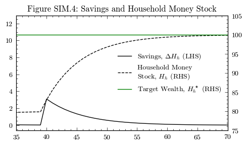
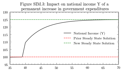
Perturbations in the Steady State

Following the convergence to the steady state, we can introduce a shock in government spending, increasing it by 5 units. Accordingly, the steady state given by \(Y^\star=\frac{G}{\theta}\) would shift to \(Y^\star=125\)

This kind of scenario can easily be implemented in the MacroStat version by adding a scenario:

1. Noting that we have convergence to the steady state at period 40, let us set this as the scenario trigger

2. We then need a new timeseries for the scenario, where \(G=25\) from the trigger period onwards

model.parameters["scenario_trigger"] = 40
model.scenarios.add_scenario(
    name="GovernmentDemandIncrease",
    timeseries={"GovernmentDemand":25}
)
model.simulate(scenario="GovernmentDemandIncrease")
output_government_demand_increase = model.variables.to_pandas()

National Income

steady_state_income_new = model.scenarios[("GovernmentDemandIncrease","GovernmentDemand")][-1] / model.parameters["TaxRate"]

fig, axs = plt.subplots(1, 1, figsize=(5, 3))
axs.plot(output_government_demand_increase['NationalIncome'], color='k', label='National Income (Y)')
axs.axhline(y=steady_state_income, color='r', linestyle='--', label='Prior Steady State Solution')
axs.axhline(y=steady_state_income_new, color='g', linestyle='--', label='New Steady State Solution')
axs.legend(loc='center right', frameon=False)
axs.set_xlim(35,70)
axs.set_ylim(95,130)
axs.set_title('Figure SIM.3: Impact on national income Y of a\n permanent increase in government expenditures')
plt.tight_layout()
plt.show()

Consumption and Wealth

steady_state_wealth_new = alpha3 * (model.scenarios[("GovernmentDemandIncrease","GovernmentDemand")][-1] * (1-model.parameters["TaxRate"])) / model.parameters["TaxRate"]

fig, axs = plt.subplots(1, 1, figsize=(5, 3))
line1 = axs.plot(output_government_demand_increase['HouseholdMoneyStock'].diff(), color='k', label='Savings, $\Delta H_h$ (LHS)')
ax2 = axs.twinx()
line2 = ax2.plot(output_government_demand_increase['HouseholdMoneyStock'], color='k', linestyle='--', label='Household Money\nStock, $H_h$ (RHS)')
line3 = ax2.axhline(y=steady_state_wealth_new, color='g', label='Target Wealth, $H_h^\star$ (RHS)')
lines = line1 + line2 + [line3]
labels = [l.get_label() for l in lines]
axs.legend(lines, labels, loc='center right', frameon=False)
axs.set_xlim(35,70)
ax2.set_ylim(75,105)
axs.set_title('Figure SIM.4: Savings and Household Money Stock')
plt.tight_layout()
plt.show()